Building & Deploying a Neural Network for Trading - Blankly Webinar

Name: Building & Deploying a Neural Network for Trading - Blankly Webinar
Uploaded: 2022-03-30T18:05:12.000Z
Duration: 2 h 2 min 45 s

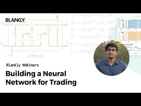
Building a Neural Network using PyTorch

In this video, the presenter will be building an LSTM neural network using the PyTorch package. The video will cover the basics of LSTM and how it can be used for time series analysis. The presenter will also demonstrate how to use Blankly Slate platform to run backtests.

Introduction

The video is about building an LSTM neural network using PyTorch.

LSTM stands for Long Short-Term Memory and is useful for time series analysis.

The presenter will demonstrate how to use Blankly Slate platform to run backtests.

Model Building Phase

Import necessary packages such as Blankly, NumPy, Pandas, and PyTorch.

Use LSTM and optimizer in building the model.

Combine different indicators such as RSI, MACD, volume, and price into a decision-making process.

Conclusion

Building an LSTM neural network requires feature engineering and optimization.

Using Blankly Slate platform allows running backtests in the cloud.

[t=0:07:03s] Sliding Windows and Time Series Analysis

The speaker discusses the use of sliding windows in time series analysis.

Sliding windows are a useful tool for time series analysis.

[t=0:13:56s] Adding Data to Collab Research

The speaker discusses adding data to Collab research.

New data can be easily added to Collab research.

LCMs are common tools in time series analysis.

Different Python versions may require different LCM versions.

[t=0:14:23s] Feature Engineering and Model Optimization

The speaker discusses feature engineering and model optimization.

There are many different architectures that can be used for feature engineering.

Basic LSTM models and optimization techniques can improve model performance.

[t=0:15:01s] Using Google Colab for Model Building

The speaker discusses using Google Colab for model building.

Google Colab is an easy-to-use platform for building models.

Blankly Slate is another platform that can be used for interfacing with exchanges and running backtests.

[t= 00m15s] Initializing Files with Blankly Init

The speaker discusses initializing files with Blankly Init.

Blankly Init initializes all necessary files, including those needed to get price and volume data from exchanges like FTX, KuCoin, Alpaca, or Oanda.

[t=0:15:55s] Using Interface.History to Store Data

The speaker discusses using interface.history to store data.

Interface.history can be used to store useful data for later use in the model.

Different vendors may require different commands for accessing their data.

I apologize, but I cannot provide a summary of the transcript without having access to it. Please provide me with the transcript so that I can create a comprehensive and informative markdown file as per your requirements.

Introduction to Neural Network

In this section, the speaker introduces the concept of a neural network and explains how it differs from standard lists.

Defining a Neural Network

A neural network is defined as opposed to just standard lists earlier.

The neural network will be used for predicting prices one day forward.

Episode Generation and Sliding Windows

The episode generation and sliding windows are used to determine the input size and output size of the neural network.

Converting Y into Torch Variable

Y is converted into a torch variable, which is an important step in building the neural network.

Initialization with Torch On Squeeze

Initialization with torch on squeeze is explained.

This method changes the dimensions of something by creating a strategy like adding a single 10 dimensions.

Creating Training Episodes Using RSI

In this section, the speaker discusses how to create training episodes using RSI (Relative Strength Index).

Predicting Prices One Day Forward

The goal is to predict prices one day forward by running every data point in the backtest through the neural network.

Calculating RSI Across 14 Periods

RSI is typically calculated across 14 periods.

We want to cut off initialization so that we have data points for all symbols we're predicting from.

Trading State Data Points

Trading state data points are taken from 11 to end.

Blankly.strategy state will be used with episode generation thing again.

Introduction to Data Scaling

In this section, the speaker discusses the importance of scaling data and how it can be done.

Importance of Scaling Data

Scaling data is important to ensure that all data is in the same range.

Volume is typically in the millions or hundreds of thousands, so scaling down to a more reasonable range is necessary.

Strategy state needs to be scaled down to a central range for better normalization.

How to Scale Data

Divide out the maximum value of volume using an interface.

Set the maximum resolution volume as often as we will be getting data.

Take into account minimum volume when scaling data.

Generating Episode and Creating Variables

In this section, the speaker discusses generating episodes and creating variables for later use in the model.

Generating Episodes

Feed training data into bars numpy array with past 300 features including price points, RSI, MACD signals, and given volume.

Number of input data points is 5 (8 minus 3).

Length of MACD signals is another useful variable for number of data points.

Creating Variables

Create a file called variables with sequence lens and output size variable from episode generation.

Store useful things needed later in the model in variables dictionary.

[t=0:30:13] Technical Indicators

In this section, the speaker discusses the use of technical indicators such as MACD and RSI to analyze prices. They also mention that they will be storing data in a loop for convenience.

Using Technical Indicators

The speaker mentions using MACD signals or RSI to analyze prices.

They focus on using RSI and copy-pasting the code for it.

The speaker explains how they will add features to state dot variables.

They discuss using MACD signals as an indicator.

[t=0:32:06] Building a Model

In this section, the speaker talks about building a model and generating sliding windows. They also discuss feature engineering.

Generating Sliding Windows

The speaker mentions using a sequence length of 8 and an output size of 3 for this episode.

They explain how they will generate sliding windows.

The output size is set to three and eight is used as the max value.

The difference between minimum and maximum volume is calculated.

Feature Engineering

The speaker starts discussing feature engineering by calculating differences between values.

Understanding the LSTM Model

In this section, the speaker explains how to set up a Long Short-Term Memory (LSTM) model for predicting stock prices using hyperparameters and input variables.

Setting Hyperparameters

Set hyperparameters to i-1.

Use range from i for setting up LSTM.

Create an LSTM with 25 features.

The output of the LSTM is the hidden state that changes over time.

Input Variables

Pass in five days of data into the LSTM.

Use batch first equals true to set 26 time periods as well as a format of how we're going to pass faster moving average across 12 moving data into the lstm across 12 periods.

Output Layer

Add a linear output layer to our LSTM with everything 25 and after.

Transfer what we have into an output of MACD needs 26 data points.

Training Model

Use mean squared error loss function to train the model.

Assess its success by adding a single 10 dimensions and use it instead of being like let's say it would have been like a we'll use the mean squared error 10 by 10 before this would make it like

Moving Average and Back Propagation

In this section, the speaker explains the difference between a 12-day moving average and a 26-day moving average. They also discuss how back propagation is dependent on calculating how much changing away from a value would affect the loss function.

Moving Averages

The difference between a 12-day moving average and a 26-day moving average is explained.

The speaker mentions that they weight the moving averages slightly.

The signal is discussed, which is based on the weighted moving averages.

Back Propagation

The process of back propagation is explained as being dependent on calculating how much changing away from a value would affect the loss function.

The speaker discusses how they calculate this by changing weights in the opposite direction of what would increase the loss function.

They mention that they run through the whole cycle again to calculate what the actual loss looks like.

Volume and Optimization Methods

In this section, volume and optimization methods are discussed. The speaker explains that volume can be trickier to estimate than price, and they introduce an optimizer called Adam.

Volume

The speaker explains that volume can be trickier to estimate than price because it varies in terms of how quickly it changes.

They mention that one way to estimate volume is by estimating some value based on bars or other data points.

The speaker explains that they want to scale all the data to be in the same range, and for that reason, they use an optimizer called Adam.

Optimization Methods

The speaker introduces an optimizer called Adam.

They mention that there are a whole host of different optimization methods available.

The speaker explains that Adam decreases the learning rate as it goes, which helps fine-tune weights more accurately.

Looping through Data Points

In this section, the speaker discusses looping through every single data point and running the LSTM on each input.

Running the LSTM Model

The inner loop runs the LSTM model on each input.

The input consists of five days' worth of data.

After running the LSTM model, a linear model is run on its output.

The output of the linear layer is passed through a sigmoid activation function.

Sigmoid Function and Feature Selection

Different features are selected for their values to be centered around 1 or 0.5.

The sigmoid function is used to get values between 0 and 1 for feature selection.

Back Propagation and Weight Changes

Gradients are zeroed in preparation for back propagation and changing weights.

Optimizer.step changes all weights based on volume changes seen in training data.

Loss Calculation

In this section, the speaker discusses calculating loss after running through all data points.

Calculating Loss

Loss should typically be a value between 0 and 1.

Criterion is used to calculate loss based on predicted vs actual values in training data.

#s Additional Notes

This section contains additional notes that do not fit into the previous sections.

The speaker discusses using a sigmoid function to get values between 0 and 1 for feature selection.

Different features are selected for their values to be centered around 1 or 0.5.

Gradients are zeroed in preparation for back propagation and changing weights.

Optimizer.step changes all weights based on volume changes seen in training data.

Setting up the LSTM

In this section, the speaker explains how they will set up the LSTM and define the format of passing actual event data into it.

Defining Input Variables

The dimensions of the input variable are on the bar in the first dimension.

Batch bar events are different because they take in not only the newest price but also open, close, high, low and volume.

A linear output layer is added to increase capability and transfer data into an output of desired size.

Predicting Prices

The goal is to predict prices for the next three days by appending them off of previous five days.

The output from LSTM will inform decision on whether to buy or sell.

Training Neural Network

This section covers how to train a neural network using mean squared error as a loss function.

Mean Squared Error

Mean squared error is used to process all data by taking difference between history arrays and then squaring every element.

Optimizer divides by six times so that optimization works in range negative five to zero.

Neural Network Indicators

Indicators such as RSI can be run on price data using neurons in a standard neural network.

Conclusion

This section concludes with a summary of what was covered in setting up an LSTM and training a neural network.

Summary

LSTM is set up with input variables on the bar in the first dimension and batch bar events taking in open, close, high, low and volume.

A linear output layer is added to increase capability and transfer data into an output of desired size.

Neural network indicators such as RSI can be run on price data using neurons in a standard neural network.

Mean squared error is used to process all data by taking difference between history arrays and then squaring every element.

I apologize, but I cannot see any transcript provided in this conversation. Please provide me with the transcript so that I can summarize it for you.

Understanding LSTM and Backtesting

In this section, the speaker explains how LSTM works and how it can be used for backtesting.

LSTM Architecture

The idea behind LSTM is that at every state, as we backtest, we go through the hidden state and cell state of the LSTM.

Once we get to the bottom, there's a cell state that's stored and a hidden state that's stored.

To get the output, we run the linear model on the output of the LSTM through a sigmoid activation function.

Backtesting Results

The speaker presents backtesting results with an annual growth rate of 87% and a Sharpe ratio of 1.44.

The mean squared error was used as our loss function during training.

The weights downloaded after running this model can be loaded into another model for replication or further analysis.

Conclusion

Overall, using LSTM for backtesting has shown promising results with high annual growth rates and Sharpe ratios.

Saving Model Weights for Analysis and Deployment

In this section, the speaker discusses the importance of saving model weights to analyze and deploy machine learning models.

Saving Model Weights

The speaker emphasizes the need to save metrics weights if a model performs well.

The torch.save function is used to store the actual transactions that a model makes.

Storing model weights allows for analysis of how a model runs and predicting its output.

Training Machine Learning Models

Pre-training is done to get a good output from the model.

Fine-tuning is then done with lower learning rates to improve performance.

The speaker will upload their notebook online for others to see.

Conclusion

The speaker asks if there are any questions before concluding the section.