Ecuaciones de Navier-Stokes

Understanding Navier-Stokes Equations

Introduction to Navier-Stokes Equations

• Salvador Madrigal and Paloma Larios introduce the topic of Navier-Stokes equations, named after French engineer Claude-Louis Navier and Anglo-Irish mathematician George Gabriel Stokes.

• The presentation will cover theoretical aspects before delving deeper into the equations with practical examples.

Characteristics of Newtonian Incompressible Fluids

• Navier-Stokes equations are partial differential equations that mathematically describe the motion of incompressible Newtonian fluids.

• A Newtonian fluid is defined by constant viscosity, which measures resistance to flow; common examples include water and air.

• An incompressible fluid maintains constant density over space and time, differentiating it from compressible fluids.

Fluid Motion Analysis

• Unlike solid objects where velocity can be determined at a single point, fluid motion requires analyzing volumes due to numerous particles involved.

• The second law of Newton applied to fluids forms the basis for understanding these equations, where mass (m), acceleration (a), and total force (F) are key components.

Mathematical Representation of Forces

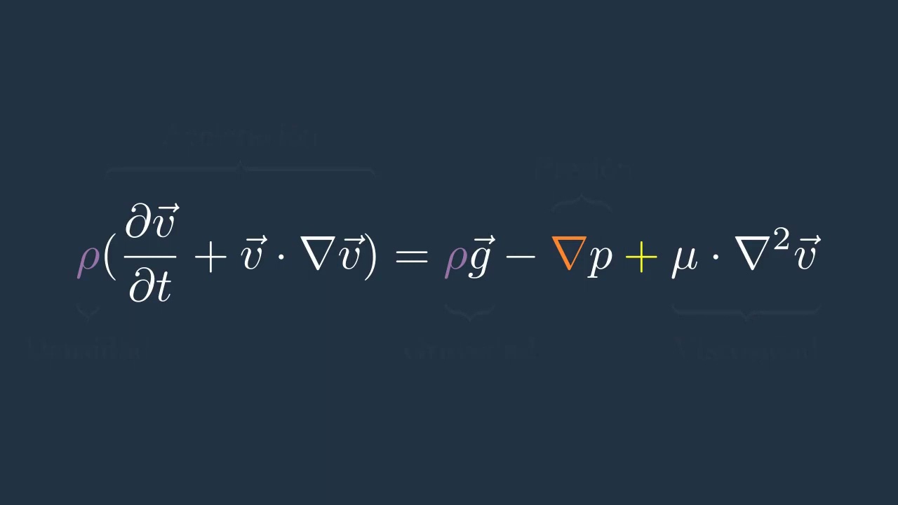
• The equation incorporates density (ρ), volumetric forces (σ), and velocity as a vector field (v).

• Total derivative expressions help in defining acceleration based on time and spatial coordinates.

Forces Acting on Fluids

• Key forces affecting fluid dynamics include gravity, pressure, and viscosity. Each force has specific mathematical definitions:

• Gravity: Defined by mass (m) and gravitational acceleration (g).

• Pressure: A function representing applied pressure at a point in space over time.

• Viscosity: A dynamic constant indicating resistance between fluid layers.

Application of Navier-Stokes Equations

• By substituting defined forces into the main equation, three separate equations emerge for describing fluid velocity in x, y, z directions.

• The divergence condition indicates that all fluid entering a volume must exit it. This principle is fundamental in deriving the complete set of Navier-Stokes equations.

Example Scenario: Flow Between Parallel Plates

Fluid Dynamics Analysis

Initial Conditions and Assumptions

• The analysis begins with the assumption of constant pressure over time, leading to zero velocity at the walls in the xy direction. This establishes initial conditions for further calculations.

• It is concluded that since pressure is a function of x, its partial derivative is a negative constant, indicating that applied force remains constant. Consequently, this results in a constant velocity in the x-direction.

Acceleration and Velocity Implications

• The acceleration in both x and z directions is determined to be zero. Thus, it follows that velocity in the y-direction also remains constant under these conditions.

• Recapping findings:

• Velocity in the x-direction does not change.

• There is no velocity component in the y-direction.

• Constant pressure implies consistent velocities across dimensions.

Differential Equations Derivation

• The focus shifts to solving differential equations for fluid dynamics:

• The equation for component i reveals static pressure behavior along y, with its partial derivative concerning x independent of y.

• Transitioning to solve for component x using initial conditions shows that changes do not depend on zeta.

Integration and Final Results

• By integrating twice based on derived equations and applying initial conditions, constants are determined.