Modelos supervisados
Exploring Supervised Machine Learning Models
Introduction to Classification Models
- The video introduces the exploration of supervised machine learning models, focusing on classification and regression.
- It highlights the importance of evaluating models and discusses metrics related to model performance, including overfitting and underfitting.
Setting Up the Environment
- The presenter connects to Azure Machine Learning workspace to access necessary resources for training.
- Key libraries mentioned include Pandas, NumPy, Scikit-learn, and Matplotlib, which are essential for developing the exercise.
Data Preparation
- The dataset used is related to diabetes, with a focus on patient information that may indicate diabetes symptoms.
- A sample of 10 records is retrieved from a DataFrame named 'diabetes' to understand the data structure better.
Understanding Variables in the Dataset
- Important variables include patient ID, number of pregnancies, plasma glucose levels, blood pressure, body mass index (BMI), and age.
- The prediction label classifies patients as diabetic (1) or non-diabetic (0), which is crucial for the classification model's function.
Training Process Overview
- The classification model aims to separate patients based on historical data regarding their diabetes status.
- Predictive variables are identified as all features except for the target variable 'diabetic', which will be predicted.
Model Complexity and Regularization
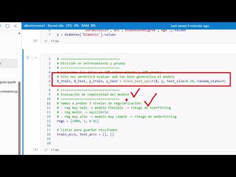
- The training process involves defining predictive variables (X-axis features) against the target variable (Y-axis).
- A split between training data (70%) and testing data (30%) is established for effective model evaluation.
Analyzing Model Performance
- Discussion on model complexity emphasizes regularization effects; high regularization can lead to underfitting while balanced regularization yields better accuracy in both training and testing phases.
Understanding Regularization in Logistic Regression
The Role of Regularization
- A regularization value of 1000 indicates a balanced model, while a value of 0.01 suggests a more flexible model that may overfit the training data.
- Overfitting occurs when the model performs well on training data but poorly on test data, leading to high training accuracy and low testing accuracy.
- The goal is to test three different regularizations (1000, 1, and 0.01) to observe scenarios of underfitting, balanced fitting, and overfitting.
Training Process
- The parameter C in logistic regression represents the inverse of the regularization strength; it helps estimate various scenarios related to regularization.
- The model is trained using logistic regression with varying values of C (1000, 1, and 0.01), allowing for predictions on both training and test datasets.
Evaluation Metrics
- Key evaluation metrics include accuracy (acurrací), precision (how many predicted positives are actual positives), recall (the sensitivity measuring true positive detection), F1 score (balance between precision and recall), and area under the curve (AUC).
- Results from each iteration are stored for graphical representation; predictions are printed for analysis across all three regularization scenarios.
Observations from Iterations
- In the first iteration with a regularization of 1000, there was evidence of underfitting with relatively low accuracies around 0.720 for training and 0.711 for testing.
- A balanced model yielded higher accuracies close to 80%: approximately 0.790 for training and 0.773 for testing.
Visualizing Results
- A graph will be constructed to visualize the relationship between regularization rates and accuracy on both training and test datasets.
- This visualization aims to compare underfitting versus overfitting scenarios effectively by displaying accuracy levels in logarithmic scale against different models' performances.