Lecture 6 - The Theoretical Minimum

Name: Lecture 6 - The Theoretical Minimum
Uploaded: 2024-09-15T12:42:18.000Z
Duration: 2 h 14 min 10 s

Understanding Photon Emission in Quantum Mechanics

Introduction to the Question

The speaker addresses a recurring question from the previous class regarding spin in a magnetic field and photon emission, emphasizing its importance.

Energy Levels and Photon Emission

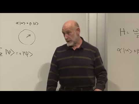
The Hamiltonian is defined as Omega/2 sigma_z , with eigenvalues of -Omega/2 (lower state) and +Omega/2 (upper state).

An energy level diagram illustrates two states: one at zero energy, another at +Omega/2 , and the lower state at -Omega/2 .

Conditions for Photon Emission

A system can emit a photon when transitioning from an upper to a lower energy state; it cannot emit if it starts in the lower state due to insufficient energy.

The emitted photon carries energy equal to the difference between the two states, specifically Omega .

Classical vs. Quantum Mechanical Perspectives

If a spin is oriented along the x-axis instead of up or down, it does not emit half-energy photons ( Omega/2 ).

Classically, a spinning rotor's energy depends on its orientation relative to the magnetic field; maximum energy occurs when aligned against the field.

Radiation Emission Dynamics

In classical mechanics, radiation is emitted continuously as an object rotates; quantum mechanically, only discrete photons are emitted.

The total emitted energy varies based on initial orientation: pointing down emits no energy while horizontal yields approximately Omega/2 .

Probabilities of Photon Emission

For superposition states (e.g., equal probabilities of being up or down), emission probability influences whether a photon is emitted.

Average emission aligns with classical expectations despite individual events resulting in either emitting a photon of energy Omega or none.

Conclusion on Absorption and Precision Requirements

Understanding Quantum Measurements and Wave Function Collapse

The Relationship Between Dipole Moment and Lifetime

The strength of the coupling in quantum systems is influenced by the magnitude of the dipole moment; a stronger dipole moment leads to faster emission rates.

There exists an uncertainty in energy levels, which is inversely related to the lifetime of the excited state, as dictated by the energy-time uncertainty principle.

Measurement Apparatus for Spin Detection

Discusses potential methods for creating apparatuses that detect electron spin, noting personal dissatisfaction with certain approaches due to their failure to meet measurement criteria.

Emphasizes that measuring a component of spin should leave the system in a specific state, raising questions about what constitutes a genuine measuring apparatus.

Wave Function Evolution and Measurement

Introduces the concept of wave function collapse during measurements, contrasting it with quantum state evolution governed by Schrödinger's equation.

Describes how external interactions (detectors or observers) influence quantum systems, leading to different states post-measurement.

Probability and State Post-Measurement

After evolving according to Schrödinger's equation, a measurement yields one specific eigenvalue from multiple possibilities; this outcome cannot be predicted beforehand.

The process of measurement does not follow Schrödinger's equation but instead depends on the nature of the measuring process itself.

Challenges with Wave Function Collapse Interpretation

While describing wave function collapse as correct, it raises concerns about having two distinct rules for system evolution: one for quantum systems (Schrödinger's equation) and another for measurements (collapse).

Questions arise regarding how to treat both system and apparatus as part of a single quantum system when considering measurements.

Combining Quantum Systems

Explores how to combine multiple quantum systems (e.g., electron spin and measurement apparatus), emphasizing that understanding this combination is crucial for accurate descriptions.

Understanding Quantum Systems and Tensor Products

The Challenge of Combined Quantum Systems

The speaker discusses the difficulty in explaining the concept of combined quantum systems, emphasizing that understanding requires thinking about both systems together.

Two systems are introduced generically as "A" and "I," with a focus on their respective state spaces, denoted as S_A for system A.

System A has states labeled by a chosen basis, while system I also possesses its own set of states, which can be expressed as superpositions of their respective basis states.

Constructing a Single Quantum System

To combine the two systems into a single quantum system, the speaker introduces the tensor product method.

The tensor product creates a new space of states for the combined system AI, mathematically represented as S_A otimes S_I .

This new space's vectors are formed by pairing off basis vectors from both systems, leading to a dimensionality defined by multiplying the dimensions of each individual state space.

Properties of Tensor Product States

The dimensionality of the tensor product is calculated as d_A times d_I , where d_A and d_I represent the number of orthogonal states in each subsystem.

Basis states in this combined system are labeled with two indices (from A and I), forming an orthonormal basis that adheres to specific inner product rules.

The inner product between different basis vectors is zero unless they match exactly; this ensures distinct observability between different combinations.

Orthonormal Basis Construction

Any choice of orthonormal bases for both subsystems will yield consistent results when constructing the combined state space.

An equation is presented to formalize how inner products behave within these bases using Kronecker delta notation to indicate when overlaps occur.

General Vectors in Tensor Products

By construction, these basis vectors form an orthonormal framework for representing any vector in the tensor product space.

Understanding Tensor Products in Quantum Systems

Introduction to Tensor Products

The concept of changing basis for individual systems corresponds to a basis change for the combined system, leading to the idea of a tensor product.

Example: Two Spins

The discussion focuses on two spins as a complex quantum system, which can be debated as one of the more complicated systems due to having four basis vectors.

Each spin is represented by an electron with three components: Sigma X, Y, and Z.

Naming Conventions

To avoid confusion with indices, the second spin is named "Tao," following Sigma in the Greek alphabet.

Tao also has three components (X, Y, Z), similar to Sigma.

Basis Vectors for Combined System

Both spins have up and down basis vectors; thus, when combined, they yield four total states: up-up, up-down, down-up, and down-down.

Each basis vector carries two labels corresponding to each spin (Sigma and Tao).

Interaction of Component Systems

While interactions may alter linear combinations of states (coefficients), they do not change the underlying basis vectors.

An example illustrates that initial states can evolve through interaction without altering their fundamental representation.

Experimental Consistency in Quantum Systems

Criteria for Experiments on Subsystems

When conducting experiments on one half of a combined system while keeping them well-separated, results should align with previous findings from treating it as an independent system.

Maintaining Correctness in Descriptions

The approach ensures that earlier descriptions remain valid even when considering subsystems together.

Exploring State Spaces vs. Observables

Direction of Discussion

A choice is presented between discussing state spaces or observables first; state spaces are chosen based on audience inclination.

Preparing States with Different Directions

Understanding Product States in Quantum Mechanics

Defining Product States

The discussion begins with the concept of a state where Sigma is aligned "up" and Tau is aligned "right," indicating a linear superposition of states.

The right direction is expressed as a combination of "up" and "down," leading to the formulation of product states involving Sigma and Tau.

A product state allows for independent preparation of two systems, where one can determine the state of Sigma while knowing Tau's orientation.

General Formulation of Product States

The most general product state can be represented as a linear combination: alpha | textup rangle + alpha | textdown rangle for Sigma, and similarly for Tau with coefficients beta.

This representation indicates that each subsystem (Sigma and Tau) can be prepared independently, reflecting their respective orientations based on detector angles.

Tensor Products and State Parameters

The relationship between these states is described as a tensor product, which combines vectors from different subsystems into a composite system.

To describe a general state vector in quantum mechanics, four complex numbers are needed; however, normalization constraints reduce this to six real parameters when considering entangled states.

Entanglement vs. Product States

It’s emphasized that not all quantum states are product states; most are entangled, requiring more parameters to describe them accurately.

In contrast to product states where individual subsystem states can be defined separately, entangled states do not allow such clear separability.

Summary Insights on Parameters

Observables in Composite Systems

Understanding Observables for Composite Systems

The observables for a composite system must align with those of the individual systems, specifically Sigma X, Y, and Z.

Operators like Sigma X act on states of the combined system by flipping states (up to down and vice versa), while remaining passive towards other indices.

When Sigma X operates on a state vector that begins with "up," it only affects the first entry and leaves the second index unchanged.

Operator Actions on States

Sigma Z returns the same state when acting on "up" but flips "down" to "-down."

Sigma Y behaves similarly to Sigma X but introduces a complex number 'i' during its operation, affecting phase without changing state direction.

Interaction Between Operators

The operator T acts similarly to Sigma operators; however, it focuses on the second entry of a state vector while treating the first as passive.

For example, T applied to an arbitrary state results in flipping between up and down states based solely on its action.

Eigenvectors in Composite Systems

Eigenvectors associated with observables remain product states of eigenvectors from individual systems; they retain their form even when considering additional degrees of freedom.

An eigenvector for a single system can be extended into composite systems by adding indices corresponding to other subsystems.

Independence of Subsystems

As long as subsystems do not interact or influence each other, they behave independently despite being part of a larger composite system.

Clarifying Misunderstandings about Operators

Operator Application Insights

Questions arise regarding whether applying an operator like Sigma X should yield superpositions; clarification is needed regarding how these operators function mathematically.

A matrix representation illustrates how operators flip states rather than maintaining them as eigenvectors.

Physical Interpretation of Non-Eigen Vectors

Applying an operator to non-eigen vectors raises questions about physical meaning; this operation often leads to orthogonal states rather than preserving original directions.

Understanding Quantum Operations and Commutativity

Auxiliary Operations and Measurement Randomness

The auxiliary operation in calculations lacks special physical meaning but indicates that measuring sigma_x in an eigenstate of sigma_z results in maximum randomness.

Product Notation and Operator Actions

Discussion on the implications of applying sigma_x to a state vector, exploring how it interacts with other operators like T_x.

Analyzing the effect of T_x on the state "up up," demonstrating how it operates selectively on components.

Order of Operations and Commutativity

Demonstrating that the order of operations between sigma_x and T_x does not affect outcomes, as shown through various examples.

Establishing that if two operators yield the same result when acting on any basis vector, they commute. This principle is illustrated with different vectors.

Independence of Subsystems

The commutation relation implies that observables from separate subsystems can be measured simultaneously without interference.

Emphasizing that measurements on one subsystem do not impact measurements on another, reinforcing their independent behavior.

Observables and Entanglement

Introduction to observables that reveal deeper connections between subsystems, such as those involving entangled states.

Clarifying that while independent systems behave separately under measurement, certain observables indicate interdependence when combined.

Product States vs. Entangled States

Distinction made between product states (where each component has its own state vector and does not interfere with others).

Understanding Entangled States

Characteristics of Non-Product States

Discussion begins on states that are not product states, highlighting their varying degrees of entanglement.

A specific entangled state is introduced: |1⟩|−⟩, noted for its unique properties, although the significance is downplayed at this stage.

Correlation Properties

The state exhibits a correlation where knowing one spin's orientation (e.g., if tow is down) determines the other's (e.g., Sigma must be up).

It is emphasized that this cannot be expressed as a product of individual states; rather, it represents a sum or difference of two product states.

Expectation Values in Quantum Mechanics

The focus shifts to expectation values of spin components in quantum mechanics and whether they can all be zero simultaneously.

The answer is revealed to be no; there always exists a direction in three-dimensional space where the expectation value for Sigma will not equal zero.

Directionality and Measurement

For any given state, there exists a linear combination of sigma components that yields a definite value (+1), indicating measurement directionality.

This leads to the conclusion that it's impossible for all expectation values to be zero since at least one direction will yield +1.

Implications for Single Spin States

When considering an isolated single spin state, it’s asserted that there exists at least one direction where the expectation value is non-zero.

The discussion transitions to examining whether any components of Sigma have non-zero expectation values in this particular entangled state.

Calculation Example with Expectation Values

An example calculation involving the inner product between different spin states and Sigma Z is presented to illustrate how these expectations are derived.

Understanding Expectation Values in Quantum Mechanics

Exploring Sigma Operators

The expectation value of the operator Sigma Z is calculated to be zero in a specific state, indicating orthogonality with other states.

When applying Sigma X, it acts as a flipper, changing the state from up-down to down-up; however, the inner product remains zero.

Similarly, for Sigma Y, which also flips states but includes an imaginary unit (i), the expectation value is found to be zero due to no common inner product.

Implications of Zero Expectation Values

The result that all three components (Sigma X, Y, Z) have zero expectation values suggests a unique property of entangled states.

This indicates that certain composite systems cannot be viewed as separate subsystems; this phenomenon exemplifies quantum entanglement.

Characteristics of Composite Systems

If one subsystem exhibits a property (like non-zero expectation), it implies similar behavior for the composite system.

An exercise is suggested to demonstrate that not all components can have zero expectation values simultaneously.

Creating Entangled States

Formation of Singlet States

A natural way to achieve entangled states occurs when two interacting spins prefer anti-alignment due to their magnetic moments.

The lowest energy configuration results from these spins being in an anti-aligned state (up-down or down-up).

Dynamics and Equilibrium

Spins will radiate photons over time and reach equilibrium in this singlet state naturally through interactions.

Factors influencing this process include proximity and strength of magnetic dipoles affecting coupling with electromagnetic fields.

Understanding Basis Changes and Entanglement

Properties of Singlet vs. Triplet States

The term "singlet" refers to its unique properties compared to triplet states; there are four basis vectors associated with these configurations.

Invariance of Entanglement

It’s confirmed that entanglement is invariant under basis changes; one can calculate entanglement entropy independent of any particular basis.

State Representation

A homework assignment involves rewriting individual spin states using left-right notation, demonstrating how structural properties remain consistent across bases.

Understanding Entangled States in Quantum Mechanics

Mixing of States

The discussion begins with the complexity of state mixing, particularly how certain states (like "up down" and "down up") can become indistinguishable when changing the basis.

It is emphasized that this mixing is not immediately obvious, indicating a deeper underlying principle at play.

Expectation Values and Observables

The speaker introduces the concept of expectation values for observables that are related to both subsystems but cannot be identified with either alone.

A specific example involving the product of operators Sigma Z and T Z is presented, highlighting the need to include factors like square roots for accurate numerical results.

Calculation Steps

The calculation proceeds by applying Sigma Z to different states, noting its effect on flipping signs rather than states themselves.

The outcome reveals an interesting result: while individual expectation values may be zero, their product yields -1, suggesting entanglement.

Insights into Entangled States

The speaker explains that despite individual measurements yielding zero for Sigma X and T X, their combined measurement leads to a consistent negative value (-1), indicative of entanglement.

This behavior illustrates that entangled states do not conform to expectations based on independent systems; they exhibit correlations that defy classical intuition.

Further Exploration of Operators

Transitioning from Sigma Z to Sigma X and T X shows similar results in terms of expectation values being -1, reinforcing the idea of strong entanglement.

The conclusion drawn is significant: these observations cannot represent a product state since such states would yield products of individual expectation values instead.

Final Thoughts on Measurements

The discussion wraps up by considering simultaneous measurements of observables. Since all sigma operators commute with each other, measuring them together reveals inherent oppositional orientations.

Understanding Spin Correlations in Quantum Mechanics

The Role of Sigma Operators

The discussion begins with the manipulation of spin states using the Sigma X operator, which flips the first entry and results in a negative correlation for certain states.

It is noted that the expectation value of Sigma X and Z components yields zero when they are not equal, illustrating a fundamental property of quantum measurements.

The speaker emphasizes that components of Sigma (X, Y, Z) are oppositely oriented, indicating a clear relationship between different spin states.

Measurement Correlations

A significant point made is that measuring one component of spin automatically informs about the opposite state of another component due to their inherent correlations.

This correlation implies that if one measures a specific component for one particle, it will yield an opposite result for its entangled counterpart.

Entangled States and Statistical Correlation

The conversation shifts to discussing entangled states as exemplified by Bell's theorem, highlighting how interactions lead to such configurations.

An analogy involving coins illustrates statistical correlations: if Alice has one coin type, Bob must have the other type without prior knowledge affecting their outcomes.

Einstein-Rosen-Podolsky (EPR) Paradox

The speaker explains that this correlation does not violate relativity; rather it reflects EPR-type correlations where measurement at one location instantaneously reveals information about another distant location.

This leads into discussions on anti-correlation where knowing one's outcome directly determines the other's state.

Classical vs. Quantum Reasoning

A distinction is made between classical reasoning and quantum mechanics; John Bell's findings challenge classical interpretations when applied to quantum systems.

The speaker asserts that attempting to simulate quantum mechanics with classical logic leads to inconsistencies in understanding quantum behavior.

Simulation Challenges in Quantum Mechanics

Quantum Mechanics and Classical Simulations

Understanding Quantum Simulation with Classical Computers

A mathematical magnetic field allows the spin to process information, where a computer solves the Schrödinger equation to determine the state over time and calculate probabilities for measurements.

An experimenter manipulating apparatuses (e.g., rotating devices, applying magnetic fields) can use a classical computer to simulate quantum mechanics, achieving results that align closely with quantum predictions through random number generation.

The described setup is not a true quantum computer; rather, it is a classical simulation of quantum behavior. Users could be misled into thinking they are conducting real quantum experiments with single electrons.

Exploring Two Spins in Separate Computers

The discussion shifts to simulating two spins located in separate computers, questioning whether it's possible for each computer to contain data for one spin while maintaining interaction.

To simulate this two-particle system effectively, continuous connections (wires) between the computers would be necessary; without direct interaction at all times, accurate simulation becomes impossible.

Non-locality and Quantum Mechanics

It is emphasized that simulating quantum mechanics locally via classical computers is unfeasible. Quantum mechanics inherently requires non-local interactions that cannot be replicated by disconnected systems.

The inability of classical computers to replicate certain aspects of quantum mechanics highlights their limitations. Quantum systems manage complex interactions without physical connections between components.