Reading and visualizing different Raster data Formats by Ravi Bhandari

Introduction to Raster Data Processing

Overview of the Session

• The session is the fourth in a series on geoprocessing using Python, focusing on raster data processing.

• Previous discussions included fundamental libraries like NumPy and Matplotlib, which are essential for handling image data.

Transition to Raster Data

• The limitations of Matplotlib's image reading capabilities for geospatial data (e.g., GeoTIFF images) are highlighted.

• Introduction of a more powerful library called "Gallal" for effective raster data processing.

Understanding Raster Data

Definition and Representation

• Raster data represents objects or variables on Earth's surface as a matrix or grid of cells, known as pixels.

• Each pixel contains values that may represent various attributes such as reflectance, temperature, or rainfall.

Bands in Raster Data

• A raster can have multiple bands corresponding to different variables; each band maintains the same structure but represents different information.

• Example: A single band might show temperature at one time point while another band shows temperature at a different time point.

Characteristics of Raster Images

Structure and Memory Representation

• Zooming into a raster image reveals its grid structure where each cell holds specific information about the area it represents.

• In computer memory, an entire raster image is stored as a matrix of numbers, making NumPy useful for processing these images.

Single vs. Multi-band Rasters

• Single-band rasters can be represented in various forms: binary images (0 or 1), grayscale images (varying shades), or classified color maps.

• Examples include digital elevation models and monochromatic images representing specific attributes like temperature at given times.

Understanding Raster Data and the Geospatial Data Abstraction Library (GDAL)

Introduction to Raster Data

• Raster images can consist of multiple bands, each representing different wavelengths across the electromagnetic spectrum, including UV, visible, and infrared.

• By combining primary colors (red, green, blue), we create a colored composite image from these bands.

Overview of GDAL

• GDAL stands for Geospatial Data Abstraction Library; it serves as a translator for various raster and vector geospatial data formats.

• GDAL is utilized for reading and writing diverse geospatial data formats, including raster data types like GeoTIFF, JPEG 2000, PNG, and others.

Features of GDAL

• Different raster formats may vary in compression methods and block sizes; GDAL abstracts these differences by providing a uniform interface.

• Regardless of the underlying format (e.g., JPEG or GeoTIFF), all images are represented through an abstract model that simplifies user interaction with the data.

User Interface and Functionality

• Users can query essential information about images such as band count, dimensions (width/height), pixel intensity data type, and projection information using GDAL.

• Unlike specific software for document types (like Microsoft Word for DOC files), GDAL supports multiple image formats under one library.

Advantages of Using GDAL

• GDAL is free and open-source software supporting over 80 image formats along with various map projections.

• It offers command line utilities alongside APIs in C, C++, Python, Java, and R to cater to different user preferences.

Community Support and Development

• Widely adopted by major geospatial data services globally; it has an active developer community contributing to its continuous improvement.

• In addition to raster support, GDAL also provides capabilities for handling vector datasets effectively.

Working with Datasets in GDAL

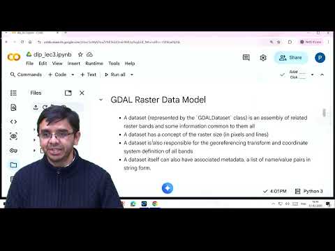
• The abstract model known as "GDAL dataset" encapsulates all necessary attributes for operating on raster images.

• This includes functions for calculating image size or fetching specific bands while managing geo-referencing transformations efficiently.

Understanding Raster Data Models and Map Projections

Overview of Raster Data Models

• The raster data model is represented graphically, where all images are encapsulated in an object called a dataset.

• A dataset can contain multiple bands, each representing different aspects of the image. Functions within the dataset allow for individual band retrieval.

• Each band contains a data array, which represents the image as a matrix of numbers. Overview bands may also be included to provide reduced resolution datasets.

Advantages of Reduced Resolution Datasets

• Reduced resolution datasets cover the same spatial extent but have larger pixel sizes, making them advantageous for viewing large areas without high computational costs.

• When zooming into an area, higher resolution images are rendered progressively to enhance detail.

Map Projection Concepts

• Map projection involves converting a three-dimensional surface (Earth) into a two-dimensional representation (map).

• Geotransformation is the mathematical process used to achieve this conversion, often resulting in some distortions depending on the projection type chosen.

Types of Distortions in Projections

• Different projections preserve various attributes: some maintain shape, others preserve area or angles; however, one must compromise on at least one aspect during transformation.

Coordinate Systems in Mapping

• A coordinate system is essential for identifying pixels on a map. Various global conventions exist for representing these systems.

• The Well-Known Text (WKT) format is one method used to represent coordinate systems within datasets.

Image Coordinate System Explained

• In an image coordinate system, every pixel is identified by its pixel number (column index) and line number (row index).

• To convert from image coordinates to real-world coordinates (latitude and longitude), geotransformation information attached to the image is utilized.

Practical Application: Reading Images with JIDAL

• For practical demonstrations using JIDAL software, users can easily install it via command line or utilize platforms like Google Colab that come pre-installed with JIDAL.

Installation and Usage of Jidal in OSJIO

Importing Jidal Module

• To use the Jidal module, first install the package named osjio. The import statement is: from osjio import jidal which allows access to the Jidal functionalities within the OSJIO package.

Setting Up Google Colab Environment

• Change your working directory to where your data is stored. This can be done by mounting your Google Drive in Google Colab, allowing for easy access to files. If not mounted, you can click an icon to do so.

• There are two methods for uploading files:

• Permanently store data on Google Drive and mount it.

• Directly upload files to Google Colab, but note that this data will be lost after a session restart or logout.

Working Directory Management

• By changing the working directory, you avoid needing to specify full file paths when accessing files during analysis. This simplifies referencing files in your code.

Inspecting Image Data with Jidal

• Use jidal.info function to retrieve basic information about an image file (e.g., geotiff). You can specify output format as JSON for structured key-value representation of metadata such as bands, block size, color interpretation, and projection information.

• The output includes details like maximum/minimum values of bands and geographic coordinates extents of the image. This provides a comprehensive overview of the image's properties.

Opening Images with Jidal

• To open an image using Jidal, utilize jidal.open, ensuring correct case sensitivity (capital 'O'). This function returns an object representing the dataset regardless of its format. Always pass the filename as a mandatory argument when calling this function.

• Once opened, various attributes and functions are available on this dataset object for further analysis (e.g., fetching width/height using raster_x_size and raster_y_size). Projection information can also be accessed through specific methods provided by Jidal utilities.

Understanding Image Geotransformation

Key Elements of Geotransformation

• The first element in the geotransformation array represents the longitude of the 0,0 pixel in a projected coordinate system measured in meters.

• The second element indicates the resolution in the X direction (e.g., 5 m), while subsequent elements detail rotation and resolution for both latitude and Y direction.

Calculating Pixel Coordinates

• To determine which area on Earth a specific pixel represents, use the built-in function jidal.apply_geotransform, passing it transformation information along with pixel and line numbers.

• This function calculates coordinates for image corners (upper left, upper right, lower left, lower right), allowing for further calculations like finding pixel centers.

Accessing Image Metadata

• Use DS.get_metadata to fetch metadata associated with an image; this can include details such as band count via DS.get_raster_count.

• Iterating through bands allows for basic statistics calculation or checking for overview bands associated with the image.

Working with Raster Bands

• Fetch individual bands from a raster dataset using get_raster_band, which returns a band object containing various functions.

• Overview levels reduce pixel size progressively; e.g., original size of 2000x2000 pixels may have overviews at resolutions of 1000x1000 down to 250x250.

Statistical Analysis of Bands

• Basic statistics such as minimum, maximum, mean, and standard deviation can be calculated across each band using band.compute_statistics.

• Setting approximation to false retrieves accurate statistical values for analysis.

Visualizing Image Data

• Images are represented as matrices of cells; fetching data involves calling ds = jidal.open(filename) followed by accessing individual bands.

• Band indices start at one in jidal (unlike numpy's zero-based indexing); use get_raster_band(1) to access the first band.

Displaying Image Arrays

• The function read_as_array retrieves data from a band as a two-dimensional numpy array representing pixel intensities.

• Visualization is achieved using plt.imshow, where you pass your two-dimensional numpy array to display the image effectively.

Image Band Visualization Techniques

Enhancing Image Quality

• The initial image quality is poor due to low contrast, necessitating enhancement for better visualization.

• Future sessions will focus on improving the image's visual appeal through various techniques.

Displaying Individual Bands

• Individual bands of an image can be displayed separately, allowing for a clearer understanding of each band’s contribution.

• The process involves iterating over the bands and visualizing them one by one, particularly in grayscale images.

Visualizing Multiband Rasters

• Satellite images often contain multiple bands (e.g., 5 to 7), but only three primary colors (red, green, blue) are needed for display on screens.

• Each band can be assigned a color: Band 1 as red, Band 2 as green, and Band 3 as blue; this creates composite images from selected bands.

Understanding False Color Composites

• Combinations of different wavelengths represented in RGB format create what are known as false color composites.

• A standard false color composite uses the near-infrared (NIR) band as red, red band as green, and green band as blue to enhance specific features in satellite imagery.

Creating False Color Composites with Jupyter

• The process begins by opening the relevant file and reading all bands together using a function that returns a three-dimensional array format (C x H x W).

• To visualize data correctly with libraries like Matplotlib, it is essential to convert from C x H x W format to H x W x C format before displaying the image. This ensures proper channel representation during visualization.

Color Composites and Data Handling in Remote Sensing

Understanding Color Composites

• Different color representations can be created by changing the band combinations of remote sensing data. For example, representing band two as red, band three as green, and band one as blue alters the visual output significantly.

• The visualization of images changes dramatically with different band combinations, allowing for the creation of false color composites that highlight various features more clearly.

• Scientists utilize these false color composites to identify distinct features in imagery, enhancing their ability to study specific characteristics effectively.

Reading Subsets of Large Datasets

• When dealing with large datasets, it is possible to read only a portion of an image by specifying pixel ranges (e.g., starting from pixel 600 and reading a 512x512 subset).

• This method allows for efficient handling of extensive data without needing to process the entire dataset at once.

Hierarchical Data Format (HDF)

• HDF is a file format designed for storing and manipulating scientific data across various systems. It consists of directories containing multiple data objects.

• Each data object within HDF has directory entries that point to its location and define its type. Two popular versions are HDF4 and HDF5.

Structure of HDF Data

• In HDF format, data is organized into groups containing datasets. Each dataset may include sub-datasets that further contain bands.

• Unlike flat file formats where bands are directly accessible, HDF organizes them hierarchically through sub-datasets.

Case Study: INSET 3DR Satellite Imagery

• The INSET 3DR satellite is designed for meteorological observations and monitoring land/ocean surfaces for weather forecasting and disaster management.

• It operates on a geostationary orbit with two payload instruments: an imager and a sounder, focusing primarily on imaging capabilities.

Imaging Capabilities

• The imager captures images from geostationary altitude using visible range cameras (0.57 - 0.72 micrometers), along with several infrared channels.

• Ground resolution varies based on the channel used; visible bands have a resolution of approximately 1 km while infrared bands range from 4 km to 8 km.

Accessing INSET 3DR Images

• Users interested in meteorological observations can download INSET 3DR images freely from the MOSDAC portal for experimentation or application development.

Continuous Monitoring Advantage

• Geostationary satellites like INSET 3DR provide continuous monitoring capabilities over specific areas every half hour, which is beneficial for applications requiring real-time updates.

How to Read HDF5 Files Using JAL

Introduction to HDF5 and JAL

• The discussion begins with an overview of images stored in HDF5 format, specifically mentioning various image timestamps (9:15, 515, etc.) and the libraries available for reading these files, including JAL.

• The speaker emphasizes that the lecture focuses on using JAL exclusively for reading images from HDF5 files. They mention changing the working directory to where the data is located.

Accessing Sub Datasets

• The main dataset in an HDF file does not directly contain bands; instead, it contains sub datasets. A function called get_sub_datasets is introduced to fetch these sub datasets.

• Each sub dataset includes a name and description. Iterating over these allows for better readability of the information contained within them.

Extracting Visual Band Data

• For demonstration purposes, the focus shifts to extracting data from a specific visual band sub dataset. The speaker explains how to pass the filename into JAL for reading.

• After opening the file with JAL, individual bands can be fetched and read as arrays.

Analyzing Satellite Images

• The speaker describes how geostationary satellites monitor areas continuously and provide surface images every half hour. This data can be used for applications like tracking cloud movement.

Creating Animations from Satellite Images

• To create animations using satellite images captured at half-hour intervals, FFmpeg is recommended as a library for generating animations from frames.

• Instructions are provided on installing FFmpeg in Google Colab and searching for relevant files in the directory containing satellite images.

Compiling Frames into a Video

• The process involves iterating through each image file, reading its data, and appending it to a list before converting this list into a three-dimensional array representing frames.

• Finally, using Matplotlib's animation package allows users to create videos by concatenating these frames together effectively.

How to Create an Animation from Frames

Defining the Update Function

• The update function is essential for continuously fetching individual frames from a combined dataset of frames, allowing for smooth animation.

• This function operates in conjunction with an animation loop that calls it repeatedly, ensuring each frame is displayed sequentially.

Converting Animation to HTML5 Video

• Once the animation object is created, it can be converted into an HTML5 video format, enabling broader accessibility and usability.

• Users have the option to export the animation as various image formats such as MP4 or JPEG after conversion.

Summary of Key Concepts Discussed

• The session concluded with a recap of reading raster images using the Jidal library, which facilitates both vector and raster data handling.

• Emphasis was placed on how raster data is represented in Jidal through a dataset object containing critical details like bands and transformation information.

Working with HDF Format

• When dealing with HDF format images, users must navigate sub-datasets to access individual bands rather than retrieving them directly from the main dataset.

Insights on 3DR Images

• The discussion included insights about 3DR images that provide Earth imagery at half-hour intervals, showcasing dynamic changes over time.