Pilot points as a model parameterisation device

New Section

In this section, the use of pilot points in parameterizing groundwater or other models with a spatial model domain is discussed.

Benefits of Highly Parameterized Inversion

• The quest for uniqueness in model calibration aims to minimize error variance in solving the inverse problem.

• Using many parameters enhances regularization, minimizing potential errors and allowing room for surprises like unexpected heterogeneity.

• Calibration serves as data interpretation through history matching, aiding in understanding underground characteristics.

Importance of Many Parameters

• Numerous parameters help analyze predictive uncertainties by capturing available information and expressing predictive uncertainty quantitatively.

• Having many parameters aids in capturing all available information and understanding the system's future behavior accurately.

Principle of Operation of Pilot Points

This section delves into the operational principles of pilot points in model parameterization.

Operational Principles

• Pilot points are assigned spatial locations with x, y coordinates (or x, y, z for 3D), distributed throughout the model domain.

• The process involves assigning values to pilot points by PEST and then interpolating from these points to the model grid or mesh.

Flexibility and Zones

• Pilot points can be associated with different zones, allowing independent interpolation within each zone without crossing boundaries.

Understanding Pest Interpolation in Model Grids

In this section, the discussion revolves around the process of interpolation from Pilot points to the model grid using PL proc within the Pest Suite.

Pest Interface with Model

• A program must run in front of the simulator to handle interpolation from Pilot points to the model grid.

• Pest writes model input files using templates and reads numbers from model output files through instruction files.

PL Proc Functionality

• PL proc (Parameter List Processor) is utilized for writing input files for the model, maintaining a non-intrusive interface with the model.

• Template files used by PL proc for writing model input files are more sophisticated, allowing for efficient transfer of large numbers during interpolation.

Interpolation Mechanisms

• PL proc can undertake interpolation from Pilot points to a model grid using various mechanisms like craing and Radial basis functions.

• It offers flexibility in applying interpolation schemes, enabling control at both horizontal and vertical levels based on different criteria.

Comparison: Craing vs. Radial Basis Functions

This part delves into a comparison between craing and Radial basis functions as interpolators within pest calibration schemes.

Craing Advantages

• Craing is numerically rapid and honors values at pilot points, minimizing undershooting or overshooting issues.

• Simple cing stabilizes extrapolation and provides mean value support, enhancing stability during modeling processes.

Radial Basis Functions Challenges

• Radial basis functions eliminate blotchiness but may result in overly smooth or unrealistic interpolated parameter fields.

New Section

In this section, the flexibility and complexity of PL proc in parameterizing a model domain through scripts are discussed.

Parameterization Flexibility and Complexity

• PL proc offers more flexibility in the parameter field compared to PE control files.

• Instructions for PL proc are scripted, akin to a programming language, allowing for complex operations like mathematical calculations between arrays.

• Detailed instructions written in files guide PL proc functions, enabling realistic interpolation and parameterization for model domains.

New Section

This part delves into handling differential densities of pilot points during model domain parameterization.

Differential Densities of Pilot Points

• Two-stage interpolation is an approach for addressing varying densities of pilot points within a model domain.

• Introduction of secondary pilot points on a finer grid allows for multipliers to perturb the background parameter field, enhancing interpolation accuracy.

New Section

The discussion shifts towards advanced interpolation techniques based on local pilot point density adjustments.

Advanced Interpolation Techniques

• Simple cing with mean adjustment facilitates stable extrapolation by fading multiplier values back to one as distance from pilot points increases.

• Background and multiplier fields interact seamlessly through simple cing, accommodating varied parameterization density across different areas efficiently.

New Section

Exploring specialized PL proc functions designed to handle variable densities of pilot points during interpolation processes.

Specialized Interpolation Functions

• Functions like Cal cing factors Auto 2D and RBF interpolate 2D automatically adjust mathematical operations based on local pilot point density variations.

Anisotropy and Parameterization in Geothermal Modeling

The discussion delves into the utilization of PL proc function to incorporate anisotropy in interpolation, focusing on elongation along valleys in geothermal modeling. It also touches upon parameterization steps involving pilot points and zones based on geological variations.

Anisotropy and Interpolation

• Anisotropy is integrated into interpolation by adjusting the direction to align with valley orientation.

• In alluvial systems, heterogeneity naturally elongates following valley directions due to deposition characteristics.

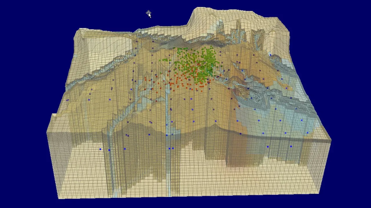
Geothermal Model Parameterization

• Creative use of PL proc in a geothermal model with a three-dimensional domain aligned with topography.

• Pilot points arranged in layers based on geological zones for effective parameterization.

Model Domain Parameterization and Calibration

The process of parameterizing a geothermal model domain involves multi-step interpolation within layers and zones, emphasizing the importance of calibration data alignment for accurate results.

Model Domain Interpolation

• Two-dimensional interpolation within layers independently followed by vertical interpolation between layers.

• Log permeability distribution colored according to permeability values post-interpolation.

Calibration Data Alignment

• Utilizing geological knowledge for comprehensive calibration data fit while maintaining model domain integrity.

• Assigning multiple parameters per layer based on hydraulic conductivity, anisotropy, storage, and head criticality.

Regression Relationships and Model Adjustment

Exploring the establishment of regression relationships between parameters for model adjustment during calibration, ensuring a balance between expert knowledge integration and data-driven adjustments.

Regression Relationship Establishment

• Establishing regression links between secondary parameters and hydraulic conductivity based on site characterization insights.

• Multi-step process involving adjustable regression lines for secondary parameters alignment with primary variables.

Model Adjustment Process

• Interpolating KH pilot point values across the model domain followed by implementing regression equations for secondary parameter assignment.

Pilot Point Placement Strategy

In this section, the speaker discusses the strategy for placing pilot points in a model domain to optimize computational resources and ensure accurate interpolation of parameters.

Pilot Point Density and Placement

• The speaker emphasizes having higher pilot point density in areas with available information to be more efficient.

• Different layers in a multi-layer model require distinct sets of pilot points for parameter interpolation to avoid excessive resource usage.

Considerations for Multi-Layer Models

• Applying the same logic of pilot point placement within each layer of a multi-layer model ensures consistency and accuracy.

• Strategic placement between observation wells based on data availability and groundwater flow direction is crucial.

Spatial Distribution Strategy

• Initiating with a budget proposal for pilot point quantity aids in parameterizing the model effectively.

• Placing pilot points where data is most needed, especially between wells, informs hydraulic conductivity estimation accurately.

Regularization Techniques for Pilot Points

This segment delves into regularization methods, specifically preferred difference regularization, to enhance inversion processes based on pilot points.

Preferred Difference Regularization

• Formulating preferred difference regularization involves linking each pilot point to its neighbors through prior information equations.

• This method promotes uniformity within the model domain or specific layers unless calibration data suggests otherwise, minimizing heterogeneity introduction.

Advantages and Challenges

• Conceptually appealing as it enforces homogeneity unless calibration data dictates variation.

New Section

In this section, the speaker discusses the challenges of regularizing parameter values in multi-layer models and introduces the concept of preferred value regularization as a solution.

Challenges in Multi-Layer Models

• The weight between layers needs to be determined, posing a challenge in achieving homogeneity within and between layers.

• Tikhonov regularization aims for homogeneity on a layer-by-layer basis but does not ensure consistency across entire layers.

Preferred Value Regularization

• Preferred value regularization offers individual fallback positions for each Pilot Point, enhancing flexibility.

• Each Pilot Point is associated with one prior information equation specifying its fallback value, addressing issues between different layers and parameter types.

New Section

This segment delves into implementing preferred value regularization using prior information equations and covariance matrices to enhance parameter estimation accuracy.

Implementing Prior Information Equations

• Assigning one equation per Pilot Point establishes individual fallback positions for each point.

• Sophistication can be introduced by estimating values for entire layers or using pilot points as multipliers with preferred values.

Adding Covariance Matrices

• The ad reg one utility simplifies adding prior information equations to a pest control file, ensuring preferred values are set accurately.

Detailed Explanation of Calibration Process

In this section, the speaker delves into the calibration process, highlighting the importance of using covariance matrices and preferred value regularization to achieve more realistic parameter fields.

Understanding Parameterization in Calibration

• The calibration process involves utilizing pilot points for two and three-dimensional models across various parameter types like hydraulic conductivity.

• Building a covariance matrix is essential but not overly challenging.

Importance of Covariance Matrix in Calibration

• Without a covariance matrix, pilot points may act independently, leading to unrealistic parameter fields.

• Using a covariance matrix alongside preferred value regularization results in smoother, more realistic parameter fields aligned with calibration objectives.

Contrasting Examples: Good vs. Bad Calibration

• A poorly calibrated model showcases blotchy parameter fields due to inadequate use of covariance matrices and regularization techniques.

• Conversely, a well-calibrated model near an open-cut pit demonstrates effective use of pilot points and preferred value regularization for accurate parameterization.

Impact of Model Orientation on Calibration

This segment explores how varying orientations of faults and dykes within a model domain influence the calibration process and the interpretation of results.

Analyzing Fault and Dyke Orientations

• Introducing faults or dykes with different conductivities reveals challenges in identifying these features through calibration alone.

• Model orientation significantly affects the visibility and interpretation of faults or dykes during the calibration process.

New Section

In this section, the speaker discusses the visibility of different geological features based on their orientation to a flow field and how regularization techniques impact model calibration.

Visibility of Geological Features

• The heterogeneity in accordance with the exponential variogram is crucial for detection.

• A conductor perpendicular to a flow field is invisible, while a resistor parallel to it is visible.

• Nonlinear regularization introduces expectations of elongation based on geological considerations.

New Section

This part delves into recalibrating models using nonlinear regularization and the implications on detecting conductive features.

Nonlinear Regularization Impact

• Nonlinear regularization guides inversion processes by imposing expected orientations.

• Geological knowledge informs the directionality of conductivity expectations.

• Calibration results reflect source signals despite pilot points' limitations in representing features accurately.

New Section

Here, the discussion centers around challenges in accurately representing structural features like faults using pilot points and regularization techniques.

Challenges in Representation

• Pilot points are limited in representing structural features such as faults or dikes accurately.

• Ticking off regularization based on variograms may not capture faults effectively.