Discrete Fourier Transform (DFT) Explained | MATLAB examples
Understanding the Discrete Fourier Transform (DFT)
Introduction to DFT and IDFT
- The presentation introduces the concept of the Discrete Fourier Transform (DFT), explaining its role in transforming signals from the time domain into the frequency domain.
- It highlights that understanding the Fourier Transform is essential before delving into DFT, as it helps identify frequencies present in a signal.
Basics of Fourier Transform
- A simple example illustrates how a sine wave at 5 Hz can be analyzed using the Fourier Transform, resulting in a clear peak at 5 Hz.
- More complex signals formed by summing multiple sine waves demonstrate that identifying individual frequencies visually is challenging, but achievable through Fourier analysis.
Defining DFT
- The DFT operates on digital data rather than continuous signals, performing similar transformations as the Fourier Transform.
- The Fast Fourier Transform (FFT) is introduced as an efficient algorithm for computing DFT, significantly reducing computational complexity.
How DFT Works
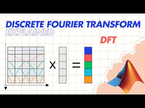
- The equation for DFT is presented; focusing on cosine terms shows how different values of k generate samples for various cosine wave frequencies.
- By multiplying each sample of a time-domain signal with corresponding cosine waves and summing them up, we can determine frequency presence within the original signal.
Spectrum Representation
- The outcome of this process yields a spectrum vector indicating strength for each cosine component present in the original signal.
- Sine components are similarly calculated using matrix multiplication to derive their contribution to the overall spectrum.
Inverse Discrete Fourier Transform (IDFT)
- IDFT allows reconstruction of an original signal from its spectrum by summing scaled sine and cosine components based on their amplitudes.
- This reconstruction can be performed either through separate synthesis matrices or via a single complex-valued transformation matrix.
Mathematical Foundations
- Equations defining both forward and inverse transformations are discussed; digitization modifies these equations from integrals to summations with discrete indices.
- Euler’s formula provides two equivalent forms for expressing DFT: exponential representation and sine/cosine representation, useful across various applications.
Conclusion and Practical Application
- The first part concludes with an invitation to explore MATLAB code demonstrating practical applications of DFT and IDFT.
Understanding DFT and IDFT in MATLAB
Generating the DFT Analysis Matrix
- The first part of the MATLAB implementation involves generating a 100 by 100 DFT analysis matrix, corresponding to the sampling frequency. The matrix utilizes an exponential form where:
- The real part represents cosine basis functions.
- The imaginary part represents sine basis functions.
Visualizing the Matrix Components
- The initial four rows of the DFT matrix are plotted, revealing:
- Real parts as cosine waves with increasing frequencies.
- Imaginary parts as sine waves, confirming expected structural properties.
Signal Spectrum Calculation
- A one-second signal with a frequency of 5 Hz is generated and plotted. Following this:
- The signal spectrum is computed by multiplying the signal vector with the DFT transformation matrix.
- Results are compared against MATLAB’s
fftfunction for validation.
- Positive frequencies appear in the first half of the spectrum vector while negative frequencies occupy the second half. To align these correctly:
- The
fftshiftfunction is employed to symmetrically reposition frequencies around zero.
Analyzing Spectrum Peaks
- Visualization of the spectrum reveals:
- A clear peak at 5 Hz, indicating its presence in the original signal.
- A symmetrical peak at -5 Hz due to properties of real-valued signals.
- Both methods (manual calculation and
fft) yield identical results, affirming their accuracy.
Reconstructing Original Signal Using IDFT
- In reconstructing the original signal from its spectrum using Inverse DFT (IDFT):
- The IDFT matrix is computed by transposing the DFT matrix, which aligns sine and cosine components appropriately for reconstruction.
- After recreating the original signal through matrix multiplication:
- Reconstruction error is calculated and visualized; results show that reconstructed signals match perfectly with originals.
- This confirms that IDFT effectively restores data with minimal error, providing a comprehensive understanding of both DFT and IDFT processes.