GT Nash equilibrium

Nash Equilibrium: Pure Strategy Overview

Introduction to Nash Equilibrium

• The lecture introduces the concept of Nash equilibrium, focusing on pure strategy Nash equilibrium.

• It highlights the tension between individual and group incentives using the prisoner's dilemma as a classic example.

Strategic Tensions

• Discusses strategic uncertainty through the battle of the sexes game, emphasizing that rationalizability does not yield unique predictions for outcomes.

• Introduces coordinated behavior as a means to achieve a single strategy profile in pure strategy Nash equilibrium.

Mechanisms for Coordination

• Suggests three stories for how players might coordinate:

• Repeated play leading to settled strategies.

• Pre-game agreements that are self-enforced.

• Mediation suggesting strategies to follow.

Revisiting Battle of the Sexes Game

• Emphasizes that rationalizability fails to predict behavior in this game, contrasting it with Nash equilibrium's focus on unilateral deviations.

Definition and Characteristics of Nash Equilibrium

• Defines Nash equilibrium as a strategy profile where no player has an incentive to unilaterally deviate from their chosen strategy while others hold theirs fixed.

• Explains best response dynamics between two players, illustrating with examples from the battle of sexes game (m,m and o,o).

Analysis of Best Responses

• Analyzes why players at m,m or o,o do not have incentives to deviate unilaterally, reinforcing their status as pure strategy Nash equilibria.

Formal Definitions of Pure Strategy Nash Equilibrium

• Provides formal definitions:

• A player's strategy must be among their best responses given other players' strategies.

• A player's payoff when playing their part must be weakly greater than any alternative strategy they could choose.

Nash Equilibrium and Best Responses in Game Theory

Understanding Nash Equilibrium

• The concept of Nash equilibrium is introduced, emphasizing that no player has the incentive to unilaterally deviate from it. Mathematically, Nash equilibria are equivalent to rationalizable strategies.

Analyzing a 3x3 Matrix Example

• A three-by-three matrix example is presented to illustrate how to identify Nash equilibria without checking every cell individually by focusing on players' best responses.

Identifying Best Responses

• When Player 2 plays strategy A, Player 1's best response is determined by comparing payoffs for strategies W, X, and Y. The highest payoff (6 for X) is underlined as the best response.

• This process continues for all strategies of Player 2; if Player 2 plays B or C while holding Player 1's strategy fixed at W, the corresponding best responses are also identified.

Finding Nash Equilibria

• Cells where both players' payoffs are underlined indicate a Nash equilibrium. In this case, (W,B) and (Y,C) are identified as equilibria since neither player has an incentive to deviate.

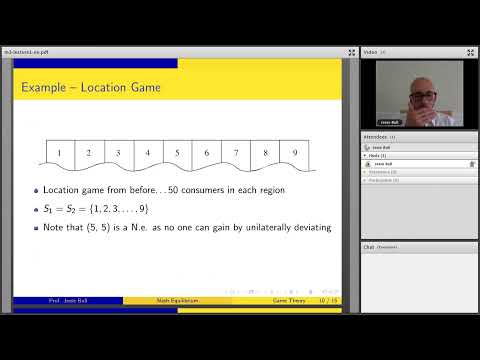
Rationalizability in Location Games

• The location game example illustrates that when both players choose strategy 5, it forms a Nash equilibrium because neither can gain by unilaterally changing their choice. This aligns with previous discussions on rationalizability.

Team Production Example: Effort Levels

• A team production scenario involves two players choosing effort levels that affect production value. Each player's effort contributes positively but incurs costs.

Calculating Marginal Costs and Benefits

• The total production value is calculated as 200 times (a_1 + a_2), while each player's cost of effort is represented as a_i^2.

• Players receive half of the total production value minus their respective costs. Thus, each player’s share becomes 100 times (a_1 + a_2).

Finding Optimal Efforts

• To find optimal efforts, marginal benefits equal marginal costs must be established. For instance, if marginal benefit equals 100, then setting this equal to 2 times a_i, leads to constant best responses of 50.

Joint Payoff Maximization Inquiry

• The discussion raises questions about whether achieving individual best responses maximizes joint payoffs in the context of shared output among players.

Understanding Nash Equilibrium and Strategic Tensions

Jointly Optimal Level of Efforts

• The marginal cost is correctly identified, with player 2's effort equating to 200 when marginal benefit equals marginal cost. This results in a jointly optimal effort level of 100 for each player.

• Players do not exert the optimal level of effort because they only receive half the benefits (100 instead of 200), leading to inefficiencies.

Inefficient Coordination in Games

• The discussion introduces a coordination game where both players prefer strategy A over B. If they match strategies, they gain higher payoffs; if not, they receive zero.

• There are two pure strategy Nash equilibria: (A,A) and (B,B). However, unilateral deviations from either equilibrium lead to lower payoffs (zero for A and one for B).

Pure Strategy Nash Equilibrium Insights

• The focus is on unilateral deviations rather than group deviations. Both players lack incentives to deviate from the inefficient equilibrium (B,B).

• A pure strategy Nash equilibrium is defined as a strategy profile where no player can gain by unilaterally changing their strategy.

Key Concepts and Skills

• Important skills include explaining three strategic tensions, defining Nash equilibrium, identifying Nash equilibria in matrix games, and recognizing them in finite normal form games or continuous strategy spaces like team production games.