Machine Learning Lecture 12 "Gradient Descent / Newton's Method" -Cornell CS4780 SP17

Understanding Logistic Regression and Naive Bayes

Overview of Logistic Regression

• The discussion begins with a recap of logistic regression, emphasizing its derivation from naive Bayes principles, focusing on learning P(X|Y) and P(Y) .

• The speaker highlights that under certain conditions, the formulation of P(Y|X) leads to a linear classifier, particularly in the Gaussian case.

• The sigmoid function is introduced as having the form 1/1 + e^-W^T X Y , which is crucial for logistic regression.

Maximum Likelihood Estimation

• The speaker proposes using maximum likelihood estimation (MLE) to optimize the likelihood for predicting P(Y|X) .

• MLE involves maximizing the product over all data points and taking the logarithm to simplify calculations.

• A specific loss function emerges from this process: minimizing log(1 + e^-W^T X_i Y_i) .

Characteristics of Loss Function

• The loss function is described as continuous and differentiable, allowing for effective optimization techniques.

• Finding the minimum point of this function is likened to high school analysis problems, reinforcing foundational concepts in optimization.

Comparison with Naive Bayes

• A critical question arises regarding why three lectures were dedicated to naive Bayes if logistic regression seems superior.

• It’s noted that logistic regression isn't always better; it can struggle with limited data due to high dimensionality leading to overfitting.

Advantages of Naive Bayes

• Two key advantages of naive Bayes are highlighted: speed (no training required compared to logistic regression's need for finding minima), and robustness with small datasets.

• Logistic regression may overfit when trained on few examples because it has too many degrees of freedom in high-dimensional space.

Practical Applications

• In spam filtering scenarios where data is scarce, naive Bayes performs better by incorporating prior assumptions about distributions (e.g., Gaussian).

• While reducing hyperplane options can be detrimental with large datasets, it helps prevent overfitting when data points are minimal.

Conclusion on Model Selection

• For initial spam filters or situations with little user interaction data, naive Bayes remains popular due to its efficiency and effectiveness.

• As more data becomes available, transitioning towards logistic regression typically yields better results.

Understanding Function Minimization

Overview of the Function

• The function measures how many points are incorrect, indicating its role in optimization.

• It is described as continuous, differentiable, and convex, resembling a bowl shape which signifies no jumps and smoothness in the function.

Initial Parameter Setting

• The initial parameter setting (W) is arbitrary; it can be set to zero or any random value.

• This initial point (W0) serves as a starting reference for optimization.

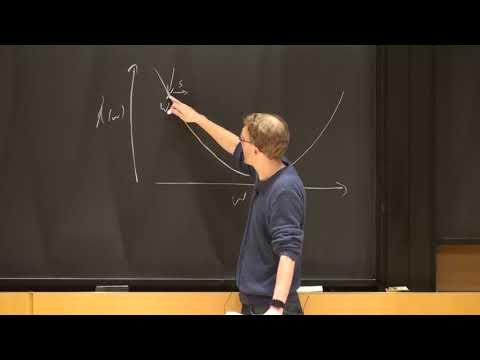
Directional Movement Towards Minimum

• The goal is to determine the direction (denoted as 's') towards the minimum of the function.

• A small step is taken in this direction to find a new point, illustrating the basic principle of hill climbing for minimization.

Challenges in Optimization

• The exact nature of the function remains unknown; it could have complex characteristics that complicate finding its minimum.

• Taking steps that are too large may lead to overshooting the minimum or landing on high loss areas.

Simplifying Assumptions for Minimization

• To tackle complexity, one assumes simpler forms like linear or quadratic functions for easier minimization.

• By fitting a line locally around W, one can identify downhill directions effectively.

Taylor's Expansion Application

• Taylor's expansion allows approximation of functions by using gradients at specific points to simplify calculations.

Understanding Function Minimization and Gradient Descent

The Role of the Hessian in Function Approximation

• The speaker discusses how considering the second term allows for a local approximation of functions as parabolas, rather than just linear functions.

• Introduces the Hessian matrix, which contains second derivatives with respect to multiple inputs, essential for understanding curvature in optimization problems.

• Emphasizes that Taylor approximations utilize first and second derivatives to create close estimates of differentiable functions.

Limitations of Taylor Expansion

• Notes that Taylor expansion approximations are valid only for small steps; larger steps can lead to incorrect minimization results.

• Explains the iterative process of minimizing using Taylor expansions: approximate, minimize, and repeat.

Gradient Descent Fundamentals

• Addresses a question about why not solely use linear approximations; mentions that while they are often sufficient, Hessians can speed up convergence in some cases.

• Defines gradient descent as a general framework for function minimization where the step size is determined by the negative gradient.

Mechanics of Gradient Descent

• Illustrates how to compute the step 's' in gradient descent as a product of the negative gradient and a small learning rate.

• Claims that taking this step will always reduce the function value if conditions (like small alpha values) are met.

Convergence Guarantees

• Discusses ensuring that each step taken leads to lower function values under certain conditions related to alpha being positive and small.

Understanding Gradient Descent and Learning Rate

The Process of Finding the Minimum

• The process of gradient descent involves iteratively moving towards a minimum point where the gradient is zero, indicating no further movement is needed.

• Questions arise about how to determine the learning rate (alpha), which must be small enough for Taylor approximation to hold true.

Challenges with Learning Rate

• A very small alpha can lead to excessively slow convergence, making it impractical for real-world applications.

• Historically, finding an appropriate alpha was considered a "dark art," with various practitioners using different methods without a clear understanding.

Modern Approaches to Learning Rate

• A safe method proposed is setting alpha as a constant divided by T (the number of updates), ensuring eventual convergence as T increases.

• Recent advancements have led to more sophisticated techniques that adaptively adjust the learning rate based on function characteristics.

Adaptive Learning Rates

• Newer methods consider the shape of the function being optimized; if steep, a smaller alpha is needed, while flatter functions may require larger steps.

• The approach involves tracking past gradients and adjusting learning rates per feature rather than using a single global rate.

Implementing Adaptive Techniques

• Each feature in high-dimensional data may require its own learning rate due to varying frequencies and importance in optimization tasks.

Gradient Descent and Optimization Techniques

Understanding Gradient Behavior

• The gradient can become very small when squared and summed over changes, leading to smaller steps in steep dimensions while allowing larger steps in shallow dimensions.

• A constant can be set for the learning rate, but it often self-regulates; thus, one can simplify by setting it to one.

Learning Rate Adjustments

• The learning rate is adjusted based on past gradients, which helps in optimizing the step size effectively.

• An epsilon value is introduced to prevent division by zero when a feature has no gradient, ensuring stability in calculations.

Stopping Criteria for Algorithms

• The algorithm should stop if the norm between consecutive weight updates is less than a small delta, indicating minimal change.

• In machine learning, precise accuracy (e.g., up to 10^-10) isn't necessary; good predictions are prioritized over exact minima.

Challenges Near Minimum

• As optimization approaches the minimum, the process slows down due to diminishing gradients. This raises questions about efficiency near convergence.

• Second-order approximations can help improve speed as they allow for more accurate adjustments close to the minimum.

Newton's Method for Fast Convergence

• By using Taylor's approximation and minimizing quadratic functions with respect to step sizes, Newton's method achieves rapid convergence.

• After each adjustment towards the minimum of a parabola derived from current weights, further iterations refine results quickly—often requiring only a few steps for high accuracy.

Matrix Gradients and Function Minimization

Understanding Newton's Method and Its Limitations

Overview of Newton's Method

• Newton's method involves taking a random vector W , computing the gradient, and multiplying it with the inverse Hessian to quickly approach function minima.

• A significant downside is that it often fails when dealing with very flat functions, as approximating them with a parabola can lead to large, inaccurate steps.

Challenges in Application

• When using Taylor approximation on flat functions, one may take excessively large steps that lead away from the minimum instead of towards it.

• An example illustrates how starting far from the minimum can result in spiraling out of control due to poor approximations by parabolas.

Recommended Approach

• It is advisable to use gradient descent initially before switching to two or three Newton steps for better convergence near the minimum.

• Some practitioners utilize only the diagonal of the Hessian matrix as an alternative second-order method or apply conjugate gradient methods for improved results.

Demonstrating Gradient Descent vs. Newton's Method

Gradient Descent Example

• A demonstration shows how different step sizes affect convergence speed; initializing at a red point leads to varying numbers of iterations based on chosen step size.

• With a fixed step size, 83 iterations were needed for convergence; however, smaller step sizes resulted in failure to converge within maximum iterations.

Impact of Step Size

• Increasing step size too much can cause divergence, illustrated by an example where excessive stepping led calculations far from the expected minimum.

Newton's Method: Advantages and Disadvantages

Benefits of Newton’s Method

• Unlike gradient descent, Newton’s method does not require manual selection of step sizes; it converges rapidly if started close enough to the minimum.

Limitations Observed

• Starting points significantly influence outcomes; beginning too far from optimal values can lead to rapid divergence despite initial accuracy.

• The ability to check for errors easily is a key advantage; if results deviate significantly after several iterations, it's clear that adjustments are necessary.

Conclusion: Practical Insights into Optimization Techniques

Summary Insights

• Understanding both methods' strengths and weaknesses allows for strategic application in optimization problems.

Gradient Descent vs. Newton's Method: A Comparative Analysis

Understanding Gradient Descent

• The speaker introduces a function they are attempting to minimize, illustrating the process of gradient descent with a black line representing its path.

• Gradient descent approaches the minimum quickly but struggles significantly in the final steps, requiring many iterations to reach precision.

• A visual comparison shows that while gradient descent makes rapid progress initially, it becomes inefficient as it nears the minimum.

Advantages of Newton's Method

• Newton's method is highlighted for its efficiency; it reaches the minimum in just a few steps compared to gradient descent.

• In scenarios where starting points are poor, Newton’s method can struggle initially, but it can be effectively combined with gradient descent for better results.

Strategy for Optimization