Real Options

Understanding Real Options

Introduction to Financial Options

• The class will focus on real options, building upon the previous discussions about financial options.

• A financial option is introduced as a key concept for understanding real options.

Defining Financial Assets and Real Options

• Financial assets are defined, setting the stage for discussing real options.

• Real options differ from traditional financial options; they involve tangible assets rather than just financial instruments.

Characteristics of Real Options

• Real options allow managers to influence project cash flows through various actions during the project's lifecycle.

• Smart managers actively seek out and create real options within their projects.

Payoff Structures: Financial vs. Real Options

• In financial options, payoffs are clearly defined by contracts (e.g., strike prices).

• Conversely, real option payoffs can vary significantly based on project circumstances.

Investment Timing Example

Scenario Setup

• An example illustrates an investment timing option involving a new telecom product that requires a $100 million investment.

Risk Assessment in Investment Decisions

• Two potential scenarios arise: high demand leading to positive cash flow or low demand resulting in sunk costs without returns.

Strategic Decision-Making with Patents

• The option to patent the device allows for one year of market research before committing significant funds.

Market Research and Demand Validation

• During this year, companies can assess market demand through prototypes and test marketing strategies.

Exercising the Option

Conditions for Investment Decisions

• If market demand appears favorable after research, the company may proceed with the $100 million investment.

Cost-Benefit Analysis of Locking in Options

• Spending $2 million to secure a patent provides valuable time to evaluate market conditions without immediate large-scale investment risks.

Analogies with Financial Options

• This scenario parallels call options in finance where exercising depends on favorable conditions (high demand).

Conclusion on Option Pricing

Understanding Real Options in Business

The Power of Option Theory

• The class focuses on applying option theory to real-world scenarios, emphasizing its relevance beyond finance majors.

• Even non-finance students can find practical examples of options in various fields, such as marketing.

Marketing and Options

• Marketing majors are encouraged to consider the phased approach when launching a new product rather than making large upfront investments.

• Initial steps include research, prototyping, and pilot studies, which serve as options that minimize risk while exploring market demand.

Understanding Real Options

• Conducting research analysis is akin to giving oneself options; it involves spending a small amount to gauge potential demand for a product.

• The term "real option" refers to physical projects where decisions are internal to an organization rather than tradable financial instruments.

Types of Real Options

Investment Timing and Expansion Options

• An investment timing option allows businesses flexibility in decision-making regarding project initiation based on market conditions.

• Example: Two businessmen set up manufacturing plants; one is rigid (A), while the other (B) purchases extra land for future expansion if demand increases.

Cost-Benefit Analysis

• Person B's additional property represents an expansion option. The cost of this option is the extra price paid for the land.

• Decision-making should be based on thorough analysis rather than blind choices; understanding costs relative to benefits is crucial.

Flexibility in Product Manufacturing

Case Study: BMW's Plant Design

• BMW built a flexible manufacturing plant capable of producing SUVs amid uncertain demand trends 15 years ago.

• This flexibility involved additional costs but allowed BMW to capitalize on rising SUV popularity without significant delays.

Strategic Planning with Options

• Smart managers incorporate options into their projects by designing work processes that allow for adaptability and value creation.

Geographic Market Expansion Strategies

Research Before Investment

• When entering new markets (e.g., Central Asia), companies should conduct preliminary research instead of immediately investing heavily in infrastructure.

Understanding Procurement Management

The Role of a Procurement Manager

• A procurement manager is responsible for purchasing goods and services for an organization, essentially acting as the buyer.

• In the context of Engrow, the biggest procurement concern is gas, which is essential for operations.

Contracting in an Integrated Market

• Gas prices are volatile; locking in a long-term contract at a fixed price (e.g., $100 per unit) can be risky if market prices fluctuate.

• If gas prices drop to $90 after signing a contract at $100, the procurement manager may regret their decision due to being locked into a higher price.

Strategic Contract Options

• To mitigate risks, smart managers include options in contracts that allow them to cancel with notice (e.g., six months).

• Offering slightly higher pricing (e.g., $100.50 instead of $100) can make it more palatable for suppliers while securing valuable cancellation options.

Value of Cancellation and Suspension Options

• Including clauses like cancellation or temporary suspension can provide immense value if market conditions change favorably over time.

• Understanding these options allows managers to negotiate better terms and potentially charge counter-parties for such flexibility.

Quantifying Business Decisions

Importance of Financial Assessment

• All business decisions should ultimately focus on financial outcomes; marketing buzzwords must translate into increased cash flow.

• Evaluating options requires understanding their financial implications—decisions must make economic sense.

Approaches to Valuing Real Options

• Various methods exist for assessing real options: discounted cash flow analysis, qualitative assessments, decision-free analysis, and Black-Scholes analysis.

Simplified Project Example

• A basic project example illustrates initial investment costs ($70 million), cost of capital (10%), risk-free rate (6%), and projected cash flows over three years.

Understanding NPV and Risk in Project Evaluation

Simplistic Assumptions in NPV Calculation

• The discussion begins with the acknowledgment that while assumptions can be complex, a simplistic approach is often used to understand concepts better. This includes considering different project timelines, such as three years versus five years.

Expected NPV Calculation

• The expected Net Present Value (NPV) of the project is calculated to be 4.6 million, emphasizing the importance of quick calculations in financial assessments.

• A specific cash flow probability of 0.3 for a cash flow of 45 is mentioned, indicating how probabilities affect expected cash flows.

Present Value and Expected Cash Flows

• The expected cash flow for each year is simplified to 30, leading to a present value calculation of expected cash flows at 74.61 million. This forms the basis for determining the overall expected NPV.

• The distinction between expected NPV and regular NPV is clarified: expected NPV incorporates probabilities of various outcomes, making it a weighted figure based on potential scenarios.

Understanding Project Risk

• The project is labeled risky due to uncertain demand; if demand falls short, it could lead to significant losses reflected in negative NPVs (e.g., a 30% chance of losing 32 million). This highlights how risk assessment plays into financial decision-making.

• An analogy comparing job security with project risk illustrates that even with positive expectations (70% chance of job retention or promotion), there remains substantial risk (30% chance of being fired). This helps contextualize risk perception in business decisions.

Options for Mitigating Risk

• A strategic option discussed involves delaying project initiation by one year to gather more information about market demand before committing resources—this reflects prudent decision-making under uncertainty.

• It’s noted that waiting does not change upfront costs or subsequent cash flows but allows for better-informed choices regarding project viability based on market research findings after one year.

Value of Real Options Under Uncertainty

• The concept that real options become more valuable when underlying projects are risky is introduced; this parallels traditional financial options where volatility increases value over time. Thus, having an option to wait enhances decision-making flexibility amid uncertainty about demand and profitability.

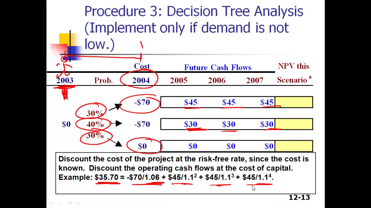
Decision Tree Analysis in Project Investment

Introduction to Decision Tree Analysis

• The session begins with a request for participants to hold their questions for the next 10 to 15 minutes, indicating an upcoming Q&A session.

Investment Options and Timing

• The analysis focuses on a project starting in 2003, where the option exists to delay investment by one year.

• Instead of investing $70 million at time 0 (2003), there is an option to invest this amount at the end of year 1 (2004).

Understanding Demand Probabilities

• At time 0, three possible demand scenarios are presented with associated probabilities.

• There is a 30% chance of high demand, which would yield cash flows of $45 million each year.

• A 40% chance exists for medium demand resulting in cash flows of $30 million each year, while there is also a 30% chance for low demand.

Evaluating Low Demand Scenario

• If low demand is confirmed at time 0, it would be unwise to invest $70 million in building the plant.

• This scenario results in an NPV (Net Present Value) of zero since no investment would occur under low demand conditions.

Calculating NPV and Discount Rates

• The NPV for high demand is calculated as approximately $35.7 based on expected cash flows discounted appropriately.

• Cash flows are discounted using different rates: risk-free rate for certain investments and higher rates reflecting uncertainty for variable cash flows.

Risk Assessment and Discounting Strategies

• Investments that are certain should use the risk-free rate; uncertain future cash flows should be discounted at a higher risk-adjusted rate (10%).

• This approach ensures conservative estimates by lowering present values through higher discount rates.

Expected NPV Calculation with Waiting Option

• To find expected NPV when waiting one year, calculations involve considering various scenarios weighted by their probabilities.

• The expected NPV from waiting is calculated as approximately $11.4, indicating increased value compared to immediate investment.

Valuing Exclusivity Rights

• If exclusivity rights must be purchased from the government, understanding maximum willingness to pay becomes crucial based on previous calculations.

• If exclusivity costs exceed potential benefits (e.g., if it costs $7 million), it would not be worth purchasing; however, if priced lower (e.g., $2 million), it could be beneficial.

Understanding Project Risk and the Option to Wait

The Impact of Waiting on Project Risk

• The option to wait can significantly alter the risk profile of a project, potentially making it less risky by eliminating scenarios with low demand.

• If low demand is identified, the decision not to invest $70 million can mitigate financial losses.

Cash Flows and Discount Rates

• Cash flows become less risky when waiting is an option, as it allows avoidance of low cash flow scenarios. However, implementation costs may still carry risks.

• A discussion arises about whether different discount rates should be applied based on project risk; lower discount rates are suggested for less risky projects.

• The exact lower discount rate remains uncertain due to limitations in finance theory.

Black-Scholes Model Introduction

• Transitioning into the Black-Scholes model, it's noted that the cost of research was not initially factored into previous calculations.

Assumptions in Financial Modeling

• Several assumptions were made during modeling: waiting for a year while spending the same amount, consistent cash flows, and no additional costs for analysis.

• These assumptions highlight potential weaknesses in the model but serve as a foundation for understanding real options.

Enhancing Financial Models

• The conversation shifts towards enhancing models by relaxing one assumption at a time—such as incorporating research costs or varying cash flows—to improve accuracy without overcomplicating analysis.

Inputs to Black-Scholes Model

Key Inputs Explained

• Essential inputs for the Black-Scholes model include exercise price (X), underlying stock price (P), standard deviation (σ), and time to maturity (T).

Understanding Each Input

• X represents the strike price; in this context, it refers to an investment of $70 million needed to initiate the project.

• P denotes the present value of future cash flows from the project rather than total NPV calculations at year zero.

Variability and Time Considerations

• σ indicates variability in cash flow projections. T reflects time until option expiration; here it's set at one year despite a three-year project duration.

Understanding Present Value and NPV

Definition of Present Value (PV) and Net Present Value (NPV)

• The price of a stock or project is defined as the present value of future cash flows, which reflects its worth.

• The value of a project is determined by calculating the present value of expected future cash flows.

Estimating Present Value

• To estimate the present value (P), one must consider the current price of the stock, equating it to the present value of expected future cash flows.

• The current price remains unaffected by exercise prices on options, emphasizing that P for real options also derives from PV calculations.

Probability and Cash Flow Scenarios

• A scenario indicates a 30% chance associated with certain future cash flows, highlighting uncertainty in projections.

• The present value at a specific point in time (2004) is noted as 111.9, illustrating how historical data informs current valuations.

Calculating Expected Values and Discount Rates

Time Considerations in Valuation

• When using a discount rate of 10%, it's crucial to apply probability-weighted numbers to derive today's price based on various scenarios.

• Clarification on whether values are calculated at time zero or one is essential for accurate financial analysis.

Discounting Future Cash Flows

• The process involves dividing by 1.1 to discount expected values back one period, yielding an estimated price today.

• This discounted figure (67.82 at time zero) serves as input for further financial models like Black-Scholes.

Variance Calculation in Financial Options

Understanding Variance

• Sigma squared represents variance; for financial options, it pertains to stock return variance while for real options it relates to project return variance.

Approaches to Estimate Variance

• Judgment-based estimation suggests that if company variance is around 10%, project variance might be slightly higher due to inherent risks.

• A direct approach will be utilized for those lacking experience, focusing on calculating variances and expected values systematically.

Final Steps in Valuation Analysis

Calculating Returns and Variance

• With established inputs including today's price (67.8), analysts can calculate potential returns based on projected prices after one year.

Methodology Recap

• Identifying possible returns from given prices allows calculation of probabilities leading to overall variance assessment.

Understanding Risk Rate and Black-Scholes Model

Exploring the Calculation of Risk Rate

• The discussion begins with identifying key variables in risk assessment, specifically focusing on "P" and "sigma squared."

• The speaker emphasizes the importance of understanding these variables to proceed with calculations.

• A suggestion is made to utilize the Black-Scholes model for further analysis, indicating its relevance in financial contexts.

• The speaker reassures listeners that they will not be required to perform manual calculations, implying a reliance on computational tools.