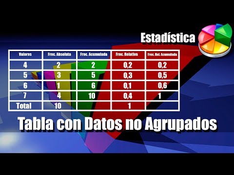
Tabla de Frecuencias para Datos no Agrupados - Ejercicios Resueltos

Understanding Frequency Tables

Introduction to Frequency Tables

• Jorge introduces the concept of frequency tables, explaining that they display how values are distributed according to their frequencies.

• The first problem involves collecting data on people's preferred beverages, which will be used to create a frequency table.

Constructing the Frequency Table

• Jorge outlines the structure of a simple frequency table with five columns, starting with listing different beverage options without any specific order.

• He begins populating the first column with beverage choices: Duff beer, Sprite, Pepsi, and Coca-Cola.

Absolute Frequencies

• Jorge explains absolute frequency as the count of how many times each beverage was chosen. For example, Duff beer was selected four times.

• He continues counting selections for other beverages: Sprite (5), Pepsi (5), and Coca-Cola (6).

Total Count Verification

• The total number of responses is calculated as 20; he emphasizes that accuracy in this column is crucial since errors affect the entire table.

• Jorge stresses the importance of double-checking counts to ensure reliability in data representation.

Cumulative Frequencies

• The next column represents cumulative frequency, which sums up absolute frequencies progressively.

• Jorge demonstrates calculating cumulative frequencies step-by-step until reaching a total of 20.

Relative Frequencies

• Moving on to relative frequencies, he defines it as the proportion of each category's count relative to the total number of responses.

• An example calculation shows that for Duff beer (4 out of 20), the relative frequency is 0.2.

Summation and Final Checks

• Jorge uses a trick by multiplying fractions by ten for easier summation and confirms that all relative frequencies add up to one.

• He concludes this section by introducing cumulative relative frequency and its calculation through progressive addition.

Conclusion from Data Analysis

Understanding Frequency Tables in Data Analysis

Introduction to Frequency Tables

• The discussion begins with the complexity of frequency tables, noting that different texts use various initial letters for terms like absolute frequency and relative frequency. The speaker opts not to include these initials for clarity.

Creating a Frequency Table

• The video introduces a practical exercise involving the creation of a frequency table based on maximum temperatures recorded throughout August. A downloadable guide with additional problems is mentioned.

• The speaker lists temperature data in degrees Celsius, starting from 15°C up to higher values, emphasizing the need to organize this data in ascending order.

Organizing Temperature Data

• The lowest temperature noted is 15°C; subsequent values are identified as 16°C, 17°C, and so forth. This organization sets the stage for constructing the first column of the frequency table.

• After identifying all unique temperature values, the speaker prepares to calculate their frequencies by counting occurrences within the dataset.

Calculating Absolute Frequencies

• Absolute frequency is defined as how many times each temperature appears in the dataset. For example, 15°C appears four times while other temperatures are counted similarly.

• Each temperature's occurrence is meticulously tallied:

• 16°C appears five times,

• 17°C also appears five times,

• 18°C shows up seven times,

• Other temperatures are counted accordingly.

Summarizing Total Frequencies

• A total count of occurrences across all temperatures leads to a final tally of 31 data points being confirmed through careful verification.

Cumulative Frequencies and Relative Frequencies

• Cumulative frequencies are calculated by summing absolute frequencies progressively. A diagonal summation technique is suggested for efficiency.

• Relative frequency represents each value's proportion compared to total observations (e.g., dividing absolute frequencies by total counts).

Finalizing Frequency Calculations

• Each relative frequency is rounded to three decimal places for precision; calculations continue until all values have been processed.

Verifying Results

• All relative frequencies should sum up to one; if they do not, it indicates an error in calculations or rounding issues.

Additional Columns: Percentages and Accumulated Frequencies

• Further columns may include percentage frequencies and cumulative percentages which provide additional insights into data distribution.

Conclusion on Frequency Table Construction

Calculating Percentages and Frequency Distribution

Understanding Percentage Calculation

• The process begins with multiplying the value 0.129 by 100%, resulting in a shift of the decimal point two places to yield 12.9%.

• The next frequency value, 0.161, is converted to a percentage as well, resulting in 16.1% after applying the same decimal shifting method.

• Additional values are calculated: 22.6% and 19.4%, completing the column of frequency percentages.

Cumulative Frequency Percentages

• To find cumulative frequencies, each percentage is summed sequentially: starting from 12.9%, then adding subsequent percentages (16.1%, etc.) until reaching a total of 100%.

• The cumulative totals are verified at each step: for example, summing up to 45.1% after including multiple values and confirming that all add up correctly to reach exactly 100%.

Analyzing Temperature Data

• The analysis reveals that the temperature recorded most frequently was 18 degrees Celsius, noted on approximately 22.6% of days.

• Conversely, temperatures of both 15 degrees and 20 degrees were less common, each appearing on about 12.9% of days.

Transitioning to Grouped Data Analysis

• The discussion indicates a shift towards analyzing grouped data in future content, suggesting an enhancement in data representation methods for better insights into temperature distributions.