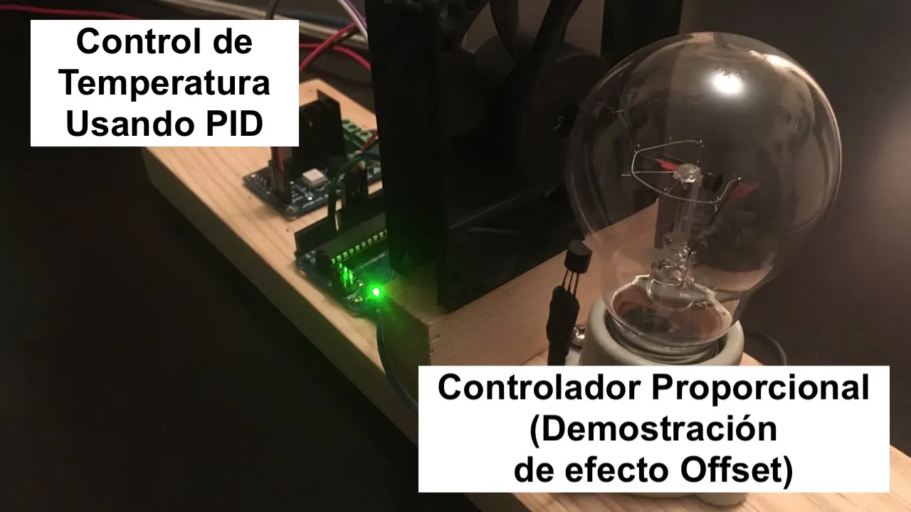
Control de Temperatura Usando PID: Controlador Proporcional (Demostración de Efecto Offset)
New Section
In this section, the speaker introduces the topic of feedback control and discusses the use of a proportional controller in contrast to a proportional-integral controller.
Understanding Feedback Control
- The speaker references a prototype setup explained in previous videos to demonstrate the application of control theory.
- Explains the concept of closed-loop systems, illustrating the difference between closed-loop and open-loop systems.
- Discusses transfer functions for closed-loop systems and introduces the concept of gain and time constant for proportional controllers.
Exploring Controller Effects
This part delves into practical applications by showcasing how specific controller values impact system behavior.
Impact of Controller Parameters
- Details experimental data used to determine process gain and time constant.
- Demonstrates the effect of setting the proportional controller value to 1 on system response.
- Analyzes system response to a step change in setpoint, highlighting issues like offset due to using a first-order system with a proportional controller.
Implementing Automatic Mode
Transitioning from manual to automatic mode while adjusting controller parameters for improved performance.
Automatic Mode Configuration
- Switches from manual to automatic mode with a high gain setting for further evaluation.
- Sets up the system with nearly equal gains for experimentation, preparing for dynamic responses.
- Initiates an experiment involving a setpoint change from 25 to 45 degrees Celsius, observing system behavior over time.
System Stabilization Analysis
Observing system stabilization and analyzing temperature responses under different operational conditions.
System Behavior Evaluation
- Monitors temperature changes over time, estimating stabilization duration based on simulation results.
Detailed Analysis of Thermal Control System Experiment
In this section, the speaker discusses the thermal control system experiment and its outcomes, reflecting on the theory versus practical application.
Understanding Temperature Control
- Theoretically, a temperature increase from 24-25 degrees Celsius should reach around 31-32 degrees after approximately 200 seconds.
Validation through Practice
- The simulation's predictions align with real-world observations, confirming the theoretical expectations.
Excitement in Practical Application
- The speaker finds this experiment one of the most thrilling due to verifying a theory in a real system, emphasizing the excitement of practical validation.
Exploring System Response to Parameter Changes
This segment delves into altering parameters within the thermal control system to observe how changes impact system behavior.
Impact of Parameter Adjustment
- Increasing a parameter value (e.g., changing 'a' to nearly 10) results in recalculations for a new transfer function with a smaller time constant.
Analyzing Graphical Representation
- A more negative pole indicates faster response times, as evidenced by simulations stabilizing around 150 seconds compared to the initial 200 seconds.
Observing System Behavior under Different Conditions
Here, the focus shifts to observing system behavior when adjusting parameters and transitioning between manual and automatic modes.
Transitioning Modes for Observation
- Adjustments are made while transitioning from manual mode (cooling down) to automatic mode (with a constant of 10), setting up for further observation.
Analyzing Controller Performance and Stability
This part explores how controller settings influence system stability and performance under varying conditions.
Controller Response Evaluation
- Observing how controller adjustments affect system behavior, noting increased aggressiveness in maintaining set points with quicker temperature changes.
Final Reflection on System Dynamics
Concluding thoughts on system dynamics and implications of parameter adjustments on stability and control efficiency.
Balancing Stability and Speed