Potential Flow Part 2: Details and Examples

Introduction to Potential Flows

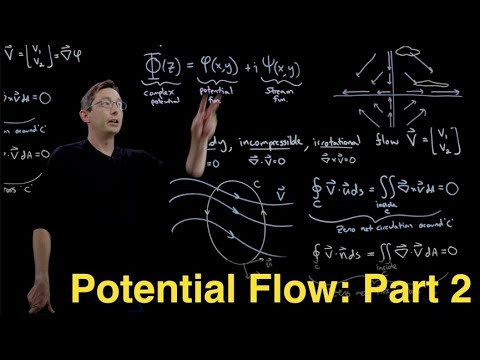
In this section, the lecturer introduces potential flows and their properties. The focus is on deriving Laplace's equation as the partial differential equation needed to find a suitable potential function.

Properties of Potential Flows

• A potential flow vector field, denoted as v, is steady, incompressible, and irrotational.

• The gradient of a scalar potential phi satisfies Laplace's equation.

• The resulting potential flow can be used to describe various phenomena in fluid flow physics.

Circulation Property

• For any closed curve C in the flow field, the contour integral of the velocity component (v) dotted into the tangential direction (u) around C is equal to zero.

• This implies that there is zero net circulation or vorticity around C for all closed curves.

Flux Property

• The contour integral of the velocity component (v) dotted into the normal direction integrated around a closed curve C is also equal to zero.

• This indicates that there is zero net flux through C.

Application of Gauss's Divergence Theorem

In this section, the lecturer discusses how Gauss's divergence theorem applies to potential flows and relates it to flux and divergence properties.

Flux Property and Gauss's Divergence Theorem

• The flux property states that there is zero net flux across a closed contour in a potential flow.

• By applying Gauss's divergence theorem, we can express this property as a volume integral inside C of the divergence of v being equal to zero.

Conclusion

In this section, the lecturer concludes by summarizing the properties of potential flows discussed earlier.

Recap of Properties

• Potential flows have the property of zero net circulation around any closed contour.

• Potential flows also have the property of zero net flux across a closed contour.

• These properties make potential flows useful in describing fluid flow phenomena.

The transcript does not provide further content beyond this point.

New Section

This section introduces the concept of potential flow and its relation to Laplace's equation. It explains that an analytic complex function can be used as a potential for potential flows, and the real and imaginary parts of these functions satisfy the Cauchy-Riemann conditions, making them solutions of Laplace's equation.

Potential Flow and Analytic Complex Functions

• Potential flow is related to Laplace's equation.

• An analytic complex function phi(z) can be used as a potential for potential flows.

• The real part (phi) and imaginary part (psi) of an analytic complex function satisfy the Cauchy-Riemann conditions.

• The real part (phi) and imaginary part (psi) are both solutions of Laplace's equation.

New Section

This section highlights the importance of complex analysis in finding solutions to Laplace's equation. It explains that taking the gradient of the real part of an analytic function gives a guaranteed potential flow, which is a cornerstone result in complex analysis.

Importance of Complex Analysis in Finding Solutions

• Taking the gradient of the real part of an analytic function gives a guaranteed potential flow.

• This is one of the most important results in complex number theory.

• Complex analysis is useful for finding solutions to Laplace's equation.

New Section

This section discusses how to derive a vector field from an analytic function using its real and imaginary parts. It also mentions that the stream function can be derived from the real and imaginary parts, providing another representation for fluid flows.

Deriving Vector Field from Analytic Function

• The gradient of the real part (phi) gives a vector field representing potential flow.

• The stream function (psi) can also be derived from the real and imaginary parts.

• The stream function is a common representation of fluid flows in fluid mechanics.

• Level sets of the stream function correspond to streamlines of the flow.

New Section

This section mentions the connection between the stream function and Hamiltonian equations of motion. It highlights that the stream function can be thought of as a Hamiltonian energy function.

Connection Between Stream Function and Hamiltonian Equations

• The stream function (psi) has a similar structure to Hamiltonian equations of motion.

• The stream function can be considered as a Hamiltonian energy function.

New Section

This section focuses on deriving the potential and stream functions for z squared. It explains how to collect real and imaginary parts, and then calculates the vector field using these functions.

Deriving Potential and Stream Functions for z squared

• For z squared, collecting real and imaginary parts gives x^2 - y^2 + 2ixy.

• The potential function (phi) is x^2 - y^2, while the stream function (psi) is 2xy.

• The vector field can be derived from these functions: v = 2x î - 2y ĵ.

New Section

This section verifies that the derived vector field is incompressible and irrotational by checking its divergence and curl respectively. It confirms that both phi and psi satisfy Laplace's equation.

Verifying Incompressibility, Irrotationality, and Laplace's Equation

• The divergence of the vector field is zero, indicating incompressibility.

• The curl of the vector field is zero, indicating irrotationality.

• Both phi (potential) and psi (stream) satisfy Laplace's equation.

New Section

In this section, the speaker discusses the properties of a function and its derivatives with respect to x and y. The function satisfies Laplace's equation and the second partial derivative sum equals zero.

Function Properties

• Taking the first derivative of the function with respect to x gives 2x.

• Taking the second derivative of the function with respect to x gives 2.

• Taking the second derivative of the function with respect to y gives -2.

Laplace's Equation

• The function satisfies Laplace's equation, which states that the sum of the second partial derivatives is equal to zero.

• The partial squared psi partial x squared plus partial squared psi partial y squared equals zero.

New Section

In this section, the speaker further explores how the stream function satisfies Laplace's equation. They demonstrate that taking derivatives of the stream function also results in satisfying Laplace's equation.

Stream Function Derivatives

• Taking the first derivative of the stream function with respect to x gives 2y.

• Taking the second derivative of the stream function with respect to x gives 0.

New Section

This section focuses on expanding an analytic function into complex variables and collecting real and imaginary parts. The resulting functions satisfy Laplace's equation.

Analytic Function Expansion

• An analytic function z squared is expanded into complex variables.

• Real and imaginary parts are collected from this expansion.

• The real and imaginary parts are functions of x and y.

• These functions satisfy Laplace's equation.

New Section

Here, we learn about how potential functions and stream functions that satisfy Laplace's equation can be used to create an incompressible and irrotational vector field.

Gradient of Potential Function

• Taking the gradient of the potential function results in a vector field.

• This vector field is incompressible and irrotational.

New Section

The speaker visually demonstrates the vector field created by the gradient of the potential function, showcasing its direction and magnitude.

Visualization of Vector Field

• The vector field is represented by arrows.

• The x-component of the vector field is 2x, while the y-component is -2y.

• Arrows point in their respective directions based on these components.

• The farther from the origin, the faster the arrows move.

• Negative directions are indicated by arrows pointing inwards.

New Section

Continuing from the previous section, the speaker explains how different unit steps in x and y affect the vector field and its direction.

Vector Field Direction

• Moving in just the x-direction results in a vector (2, 0).

• Moving in just the y-direction results in a vector (0, -2).

• As one moves farther along either axis, arrow magnitude increases accordingly.

• At specific points like (1, 1), vectors move diagonally with components (2, -2).

New Section

The speaker describes how this particular vector field behaves like a saddle function. They explain how it stretches out in one direction while compressing in another.

Saddle Function Behavior

• The shape of this vector field resembles that of a saddle.

• It stretches out along one axis (x) and compresses along another axis (y).

• This behavior creates an incompressible and irrotational flow.

New Section

In this section, we learn about how particles flow through the vector field and how certain properties are preserved during this flow.

Flow of Particles

• Dropping a blob of mass into the vector field results in stretching along the x-axis and compression along the y-axis.

• The total area of the blob remains constant as it flows through the field.

• This preservation of closed areas is due to the divergence being zero.

• The orientation of objects remains conserved during this flow.

New Section

The speaker emphasizes an important concept in vector calculus and partial differential equations. They explain how solutions to PDEs define vector fields, which can be thought of as ordinary differential equations for particles in that field.

Vector Fields and Particle Motion

• Solutions to PDEs often define vector fields.

• These vector fields can be seen as ordinary differential equations for particle motion.

• A three-step process involves: 1) having a PDE, 2) obtaining a vector field, and 3) considering particles moving within that field.

• Examples like the Navier-Stokes equation demonstrate this concept.

New Section

The speaker reiterates the three-step process mentioned earlier, emphasizing its significance in understanding partial differential equations, vector calculus, and fluid flows.

Three-Step Process

1. Start with a partial differential equation (PDE).

2. Obtain a corresponding vector field (v).

3. Consider particles moving within that vector field as an ordinary differential equation (ODE).

New Section

In this section, we learn about how solutions to PDEs can result in unsteady, compressible, and rotating vector fields. The concept of integrating particles through these fields is introduced.

Solutions to PDEs

• Solutions to PDEs can result in vector fields that are unsteady, compressible, and rotating.

• The Navier-Stokes equation is an example of such a PDE solution.

• Particles can be dropped into these vector fields and integrated along their paths.

New Section

The speaker concludes by summarizing the importance of understanding partial differential equations, vector calculus, and flows. They emphasize the concept of particles moving within vector fields as ordinary differential equations.

Importance of Understanding

• Understanding partial differential equations, vector calculus, and flows is crucial.

• Integrating particles through vector fields helps comprehend fluid dynamics.

• The three-step process provides a framework for analyzing PDEs and their solutions.

Understanding the Structure of Flow in the Ocean

In this section, the speaker discusses how studying particle movement in the ocean can provide insights into the flow structure. The Navier-Stokes vector field is introduced as a tool to predict and analyze particle movement.

Flow Structure and Particle Movement

• Pollution dropped in the ocean helps identify flow patterns.

• Integration of particles through the Navier-Stokes vector field predicts their movement.

• The vector field represents a solution to a partial differential equation.

Saddle Point Analysis

• The vector field resembles a saddle shape.

• It can be represented as a matrix form of an ordinary differential equation.

• The origin serves as a fixed point, making it a saddle point.

Eigenvalues and Eigenvectors

• The linear ordinary differential equation has eigenvalues (+2, -2).

• Eigenvectors correspond to these eigenvalues in x and y directions.

• A potential function satisfying Laplace's equation describes particle behavior.

Potential Flow and Ocean Gyres

• Potential flow models complex fluid flows like ocean gyres.

• Ocean gyres consist of counter rotating basins with chaotic mixing potential.

• A stream function, such as psi(x,y) = sin(pix) * sin(piy), can represent this flow pattern.

Modeling Counter Rotating Ocean Gyres

This section focuses on modeling counter rotating ocean gyres using potential flows. The stream function is used to create a box with two large vortices that rotate in opposite directions.

Counter Rotating Vortices

• Two large vortices rotate in opposite directions within a box.

• An approximate potential flow solution captures this counter rotating motion.

Stream Function Representation

• The stream function psi(x,y) = sin(pix) * sin(piy) represents the potential flow.

• The vector field derived from the stream function satisfies specific partial derivatives.

Visualization and Analysis

• Plotting the streamlines or level sets of the vector field reveals the counter rotating ocean gyre pattern.

• Dropping particles into this flow allows for studying stretching and mixing behavior.

Potential Flow and Analytic Functions

This section explores the relationship between potential flows and analytic functions. It highlights how various complex functions can generate potential or stream functions, which are essential for designing aircraft wings.

Relationship to Analytic Functions

• Potential flows are obtained from analytic complex functions.

• Polynomial, trigonometric, exponential, and logarithmic functions can establish these flows.

Harmonic Solutions of Laplace's Equation

• Complex functions with real and imaginary parts that satisfy Laplace's equation provide potential or stream functions.

• These solutions offer an infinite family of vector fields with desirable properties.

Application in Aircraft Wing Design

• Potential flows derived from analytic functions were traditionally used in designing aircraft wings.

• By combining these building blocks, engineers could create desired flow features for optimal lift and drag properties.