Divergence Operator in Vector Calculus

Introduction to Divergence

• The lecture focuses on the divergence operator, a key vector calculus operation used to describe physical systems and partial differential equations.

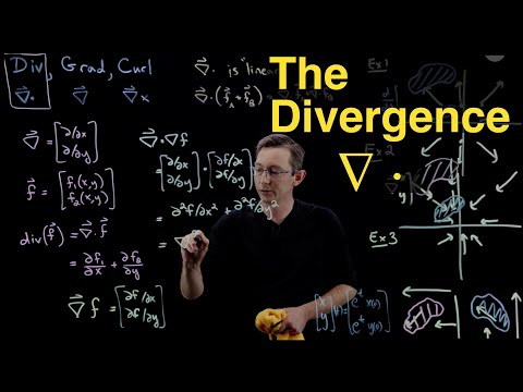
• The divergence operator is introduced as part of the noblah (or Dell) operator, which consists of partial derivatives in two dimensions.

Understanding the Divergence Operator

• The divergence involves taking the dot product of a vector field with a vector of partial derivatives, resulting in a scalar function.

• When applying the divergence to a vector-valued function f , it yields a scalar value representing how much the vector field is sourcing or sinking material locally.

Physical Interpretation of Divergence

• A zero divergence indicates no net local compression or expansion within the vector field, while positive or negative values indicate sourcing or sinking behavior.

• The linearity of the divergence operator is emphasized; it allows for additive properties when combining multiple vector fields.

Examples and Applications

• Three examples are provided to illustrate practical applications of divergence. The first example features a simple vector field defined by f(x,y) = xhati + yhatj .

• This example demonstrates that at every point in space, there exists a corresponding vector indicating direction and magnitude based on coordinates.

Computing Divergence: Example 1

• Visual representation shows vectors diverging from the origin, suggesting positive divergence due to outward movement.

• Calculation reveals that textdiv(f) = 2 , confirming that this flow has positive divergence and thus expands over time.

Divergence in Vector Fields

Example of a Converging Vector Field

• The example illustrates a converging vector field defined by the function f(x, y) = -x hati - y hatj . This represents vectors pointing inward towards the origin.

• The direction of the arrows has been reversed compared to previous examples, indicating that points move toward the origin with increasing speed as they are farther away from it.

Computing Divergence

• To compute divergence, take the dot product of the partial derivative vector with the vector field: textdiv(f) = partial (-x)/partial x + partial (-y)/partial y . This results in a divergence value of -2.

• A negative divergence indicates that volumes are contracting, which is characteristic of compressible flow where things are converging rather than diverging.

Characteristics of Divergence

• Positive divergence implies volume growth, while negative divergence signifies volume contraction. The example demonstrates how patches in space shrink over time due to negative divergence values.

• The next example will illustrate a vector field with zero divergence, where volumes remain constant over time.

Example of Zero Divergence Vector Field

• The third example features a vector field defined by f(x,y) = -y hati + x hatj , differing from previous fields as its components are switched. This setup leads to unique rotational behavior without expansion or contraction.

• Evaluating this vector at various test points shows directional changes; for instance, at (1,0), it points up (0,1), and at (0,1), it points left (-1,0). Thus illustrating complex movement patterns within this field.

Confirming Zero Divergence

• To confirm zero divergence: textdiv(f) = 0 + 0 = 0. This means that this vector field is "divergence-free," characterized solely by rotation without any sourcing or sinking behavior.

• When observing a patch in this flow, it remains unchanged in size but rotates around its center point over time—demonstrating solid body rotation characteristics typical for divergence-free fields.

Implications and Applications

• Understanding these concepts allows us to view vector fields as establishing differential equations governing particle motion within those fields: DDT(x,y) = F(x,y) . This perspective aids in analyzing systems dynamically through their respective flows.

Understanding Divergence and the Laplacian in Vector Fields

The Concept of Divergence

• The divergence is defined as the dot product of the del operator with a vector-valued function, connecting it to the exponential expansion rate of particles in vector fields.

• When calculating the divergence, the result is a scalar function. For linear vector fields, this results in a constant scalar; however, if modified (e.g., using x^2), it becomes a function of x.

• The divergence can indicate local behavior in a vector field: whether particles are expanding, contracting, or exhibiting solid body rotation (divergence-free).

Gradient and Its Divergence

• Taking the gradient of a scalar function transforms it into a vector-valued function. This involves computing partial derivatives with respect to each variable.

• The divergence of this gradient leads to an important mathematical expression involving second partial derivatives. Specifically, it combines these derivatives into one quantity.

Introduction to the Laplacian

• The result from taking the divergence of the gradient is known as the Laplacian (nabla^2 f). It represents a scalar value derived from second partial derivatives.

• The Laplacian is crucial across various physics applications such as studying electrostatic potentials and fluid flows. It serves as an essential tool for solving partial differential equations.

Building Blocks in Vector Calculus

• Understanding how to compute gradients and divergences allows for effective manipulation of functions within physics contexts. The relationship between scalars and vectors through these operations is foundational.

Upcoming Topics