อัลกอริทึม : 2.11 การวิเคราะห์ - การทำงานแบบเรียกซ้ำ
Understanding Recursive Algorithms
Introduction to Recursion
- The concept of recursion is introduced, highlighting its structure where a problem is broken down into smaller instances.
- A base case is defined for small input sizes that can be solved directly, returning results immediately.
- The analysis of algorithms involves defining T(n), where n represents the size of the input data.
Analyzing Algorithm Performance
- The algorithm's performance is divided into two parts: non-recursive processing and recursive calls with reduced input size.
- Recursive definitions are established based on how the input size decreases, such as n/3 or n - 10.
Importance of Correctness in Recursion
- Emphasizes that incorrect assumptions in defining the recurrence relation will lead to flawed analysis.
- Once a correct recurrence relation is established, mathematical techniques are used to solve it for closed-form expressions.
Example: Binary Search Algorithm
- Introduces binary search as an example of a recursive algorithm, focusing on searching for an element x within a range defined by left and right indices.
- Defines edge cases where no elements exist (left > right), leading to an immediate return value indicating failure (-1).
Implementing Binary Search Recursively
- Describes how to calculate the middle index and check if it matches the target value x.
- If x is less than the middle value, search continues in the left sub-array; otherwise, it searches in the right sub-array.
Defining Input Size for Binary Search
- Clarifies that only elements between left and right indices are considered when determining input size M.
- Establishes M = Right - Left + 1 as a formula for counting elements within the specified range.
Writing Recurrence Relation for Binary Search
- Defines TM as time complexity based on searching M elements recursively with TM/2 representing halving the search space each time.
Understanding Recurrence Relations in Binary Search
Introduction to Recurrence Relations
- The discussion begins with the foundational commands of recurrence relations, emphasizing that there are no loops involved. This sets the stage for understanding how binary search operates over time.
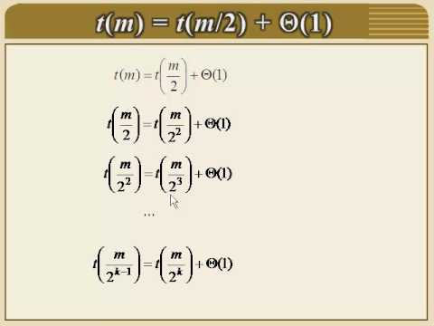
- The speaker introduces a method for solving recurrences by gradually substituting values, referring to this technique as "unfolding." This approach simplifies the complexity of the recurrence.
Deriving the Formula
- A specific example is provided where TM (time complexity) is expressed in terms of M squared and T1, leading to a derived formula involving powers of 2.
- The process continues with substitutions that lead to a general form: TM = TM(2^k - 1). The importance of determining k is highlighted, as it indicates how many iterations or lines are involved in the binary search.
Analyzing Time Complexity
- As equations are combined, redundant terms cancel out, leaving only significant components like TM and constants. This simplification aids in understanding overall time complexity.
- The speaker emphasizes that if M equals zero at some point, it implies certain conditions about K's value. Establishing this relationship helps clarify how many operations will be performed.
Finalizing Time Complexity
- By taking logarithms on both sides of an equation involving M and K, a final expression for K emerges: K = 1 + log2(M). This leads to insights about operational limits during searches.
- It’s concluded that when searching fails (i.e., finding zero elements), the time taken aligns with O(log M), establishing a clear boundary for binary search efficiency.
Exploring Hanoi Tower Problem
Overview of Hanoi Tower Algorithm
- Transitioning from binary search, the speaker introduces the Tower of Hanoi problem as another example where recursive analysis applies.
- Here, n represents disks; moving these disks involves recursive calls which can be analyzed similarly to previous examples.
Recursive Structure Analysis
- The recurrence relation for Hanoi is established: Tn = 2T(n - 1) + C1. Each move reduces disk count by one while doubling operations due to two recursive calls.
- Emphasis is placed on identifying non-recursive work done during each call—this includes constant-time operations not dependent on n.
Solving Recurrence Relation
- When analyzing minimal cases (e.g., zero disks), it's noted that no moves are required. Thus T0 = C0 signifies base case handling within recursion.
Resulting Time Complexity
Understanding Recurrence Relations
Substituting Values in Recurrence Relations
- The process begins with substituting values into the recurrence relation, specifically tn - 1 = 2 cdot tn - 2 + c_1 . This substitution leads to a new expression that simplifies further calculations.
- After substitution, multiplying by 4 yields results such as 4 cdot 2 = 8 , and this pattern continues as each term is expressed in terms of powers of 2.
Identifying Patterns in Powers of Two
- Observations reveal that the coefficients can be represented as powers of two: 8 = 2^3 , 4 = 2^2 , and so forth. This establishes a clear relationship between the coefficients and their respective powers.
- The general form emerges from these observations, indicating that for any n, the sequence will conclude at zero when there are no more items left to process (i.e., T_n = T_0 ).
Summation of Powers of Two
- A mathematical principle states that the sum of powers from 2^0 to 2^n equals (2^n+1 - 1) . This foundational knowledge aids in simplifying expressions derived from previous steps.