The Magic Formula for Trading Options Risk Free

Understanding the Breeden-Litzenberger Formula

Introduction to Risk Neutral Probability Density Functions

• The video introduces the Breeden-Litzenberger formula, which is used to derive risk-neutral probability density functions from option prices. This method is particularly useful for complex dynamics and high-dimensional scenarios.

Advantages of the Breeden-Litzenberger Formula

• The formula allows for the computation of complicated derivatives at different strikes for a specific time to maturity, simplifying the process of obtaining risk-neutral probability distributions.

Smoothing and Cumulative Density Function Creation

• After obtaining a discrete probability density function (pdf), linear regression will be applied to smooth this function, leading to the creation of a cumulative density function that facilitates easy pricing of complex derivatives.

Definition and Pricing Mechanism

• The Feynman-Kac analysis helps define risk-neutral probabilities necessary for option pricing. A European call option's price can be expressed in terms of its strike price and time to maturity using these probabilities.

Deriving Option Prices Using Integrals

• The call option price is derived through an integral involving the risk-neutral pdf, where it represents discounted expectations based on potential payoffs above a certain strike price.

Exploring General Densities Beyond Log-Normal

Transitioning from Log-Normal Distributions

• While constant volatility leads to log-normal densities yielding Black-Scholes formulas, more general densities can be considered under no-arbitrage conditions using the Breeden-Litzenberger framework.

Derivative Calculations for PDF Extraction

• Taking derivatives with respect to strike prices allows extraction of both first and second derivatives from integrals, ultimately leading to identification of the risk-neutral pdf.

Practical Application in Python

Setting Up Python Environment

• The video discusses setting up a Python environment with libraries such as NumPy, SciPy, Pandas, and Matplotlib for implementing calculations related to risk-neutral distributions.

Stochastic Volatility Model Overview

• A European call option with stochastic volatility modeled under Heston's framework is introduced. Key parameters include drift and diffusion terms relevant for underlying processes.

Parameter Initialization in Heston Model

Defining Key Parameters

• Initial parameters are set: stock price at 100, strike at 150, one-year time frame (tau), and an annual risk-free rate of 6%.

Mean Reversion Rate Considerations

• Parameters like kappa (mean reversion rate), theta (long-term variance), initial volatility values are defined while ensuring conditions are met to avoid negative volatility issues within Heston’s model framework.

Understanding Option Pricing and the Heston Model

Finite Difference Approximation for Derivatives

• The discussion begins with the application of a discount factor multiplied by the probability density function (pdf) to approximate option pricing.

• Call prices are calculated for various strikes, ensuring an even difference between them, which is essential for risk-neutral distribution calculations at specific maturities.

Analytical Solutions in the Heston Model

• An analytical solution exists for calculating option prices under the Heston model, relying on its characteristic equation. A previous video provides detailed steps on this calculation.

• Complex integrals from 0 to infinity of the characteristic function must be computed using rectangular integration methods.

Numerical Integration Challenges

• The choice of step size in numerical integration significantly affects precision, especially for out-of-the-money options due to Python's round-off errors.

• The speaker notes that C-based libraries like QuantLib are more effective than Python for numerical integration tasks.

Implementation of Rectangular Integration

• After calculating option prices using rectangular integration across a range of strikes (60 to 180), second-order finite difference approximations are employed to derive risk-neutral distributions.

• The process involves creating a data frame with strike prices and applying shift functions in Pandas to compute necessary values.

Visualization and Comparison with QuantLib

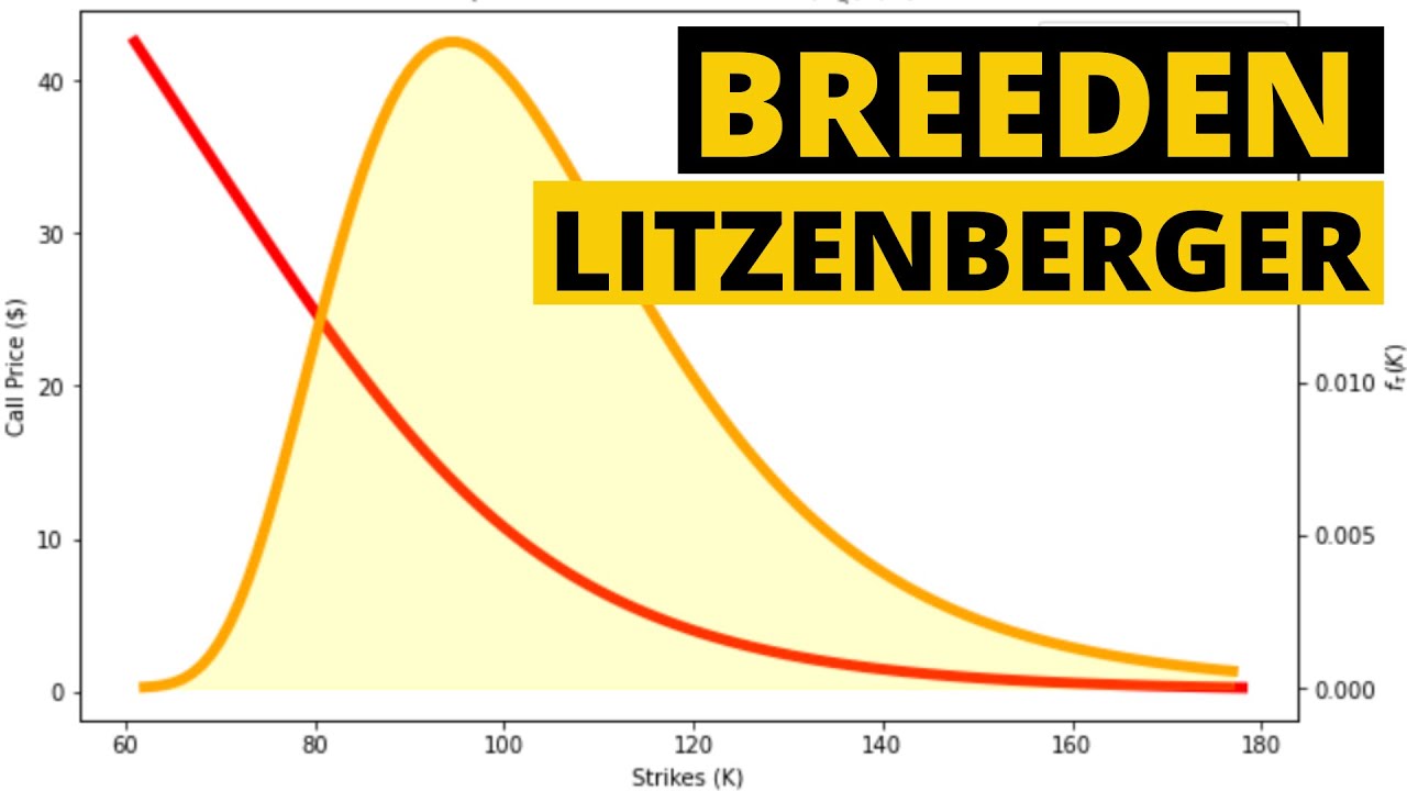
• A plot illustrates Heston stochastic volatility-calculated option prices alongside curvature representing density functions; issues arise when curvature dips below zero due to round-off errors.

Understanding Probability Density Functions and Numerical Integration

Overview of Probability Density Function (PDF) and Mean Squared Error (MSE)

• The discussion begins with the importance of a probability density function, highlighting that the density should not drop below zero, which is ideal for its application.

• The mean squared error (MSE) between option prices from rectangular integration and the QuantLib library is noted to be very small at 0.07 across various strikes, indicating minimal differences in pricing.

• Larger discrepancies occur for out-of-the-money options due to complex integration over small increments, leading to rounding errors in Python's binary float point number approximations.

Challenges with Python's Numerical Integration

• Python's limitations regarding numerical integration are discussed, particularly concerning round-off errors when dealing with small values.

• A call for suggestions on improving Python’s numerical integration methods is made, emphasizing variable step sizes for different strikes.

Interpolation Techniques for PDF Calculation

• The speaker plans to multiply option prices by a forward factor and use SciPy's interp1d function to interpolate between discrete curvature functions based on given strikes.

• It is emphasized that interpolation can only be performed within the range of provided data points; thus calculations are limited between specified strike values.

Cumulative Distribution Function (CDF)

• To derive the cumulative distribution function from the PDF, a cumulative sum of the linear PDF across all strikes is computed.

• The resulting CDF represents risk-neutral distribution at a specific time to maturity, allowing users to input a strike price k to obtain probabilities.

Pricing Complex Derivatives Using Risk-Neutral PDFs

• The risk-neutral density function can be utilized for pricing derivatives at a defined time to maturity using market prices or models like Heston’s model.

• A generic pricing formula for calls and puts is introduced, detailing how numerical integration applies to these payoffs based on stock price S_t .

• Integrands are defined for both call and put options; however, practical limits exist due to maximum calculable CDF values derived from interpolation techniques.

Understanding High-Dimensional Pricing Models

Efficiency in Pricing Calculations

• The discussion highlights the complexity involved in calculating pricing for different strikes, especially when dealing with high dimensions and time steps.

• It emphasizes that high complexity is required for accurate calculations, which can be model-dependent.

• The use of risk-neutral density functions is presented as a highly efficient method for pricing options.