Computational Plasticity (Algorithm for Mises UMAT)

Name: Computational Plasticity (Algorithm for Mises UMAT)
Uploaded: 2022-04-11T00:00:00.000Z
Duration: 20 min 45 s

Introduction

In this video, the basics of computational plasticity and the algorithm used to solve Misses equations are explained. The Miss yield function is reviewed, and the relationships between stress tensor, hydrostatic pressure, divitoric stress, and effective stress are discussed.

Basics of Computational Plasticity

The video is part two of a series that explains how to write your own first plastic unit subroutine.

The Miss yield function is the most common plastic constitutive behavior.

Effective plastic strain is defined by the plastic strain tensor.

To numerically solve the presented equations of misses plasticity we need to consider that solving of plasticity problems is incremental so we use these equations to solve an increment.

Algorithm for Solving Misses Equations

We need to calculate elastic and plastic parts of the strain increment in order to calculate stress and strain at the end of an increment.

Elastic relationships of a material are investigated assuming it's linear and isotropic using Hooke's law.

Stress and strain can be written as arrays with six components based on shear stresses or engineering shear strains respectively.

Stress increment in elastic strain increments can also be related in the same way using Hooke's law.

Elastic stiffness matrix can be written based on shear modulus G and lambda constant which can be expressed based on E (Young's modulus), nu (Poisson's ratio), or bulk modulus.

Calculation of Normal Stresses Components

For normal stresses components delta ij term should be added to the relationship where delta ij is Kronecker delta which is one for normal stresses and zero for shear stresses.

Some of the normal strains can be replaced by trace of the strain matrix.

Calculation of Elastic Strain at the End of Increment

Elastic strain at the end of an increment is written based on the strain at the beginning, total and plastic strain increments.

Elastic Predictor and Plastic Corrector

In this section, the speaker explains the role of elastic predictor trial stress and plastic corrector in calculating stress at the end of an increment. The speaker also shows how to obtain delta p by solving a vector equation.

Elastic Predictor Trial Stress

The first part of the equation is equal to the stress in the beginning of the increment plus stiffness matrix multiplied by the total strain increment.

If we assume that the strain increment is totally elastic, we can calculate the stress at the end of the increment by this equation.

This term is known as elastic predictor trial stress.

Plastic Corrector

The next term considers the plastic part of the strain increment.

We can write the plastic strain increment based on normality hypothesis.

This term is known as plastic corrector.

Role of Trial Stress and Plastic Correction

There are three situations:

Material is elastic at beginning and trial stress is also elastic. In this case, there's no plastic strain increment and final stress equals trial stress.

Material is plastic at beginning but trial stress may locate outside yield surface. Plastic corrector brings it to yield surface.

Material is elastic at beginning but trial stress locates outside yield surface. Final stress located on yield surface by plastic corrector.

Obtaining Delta P

To obtain delta p, we need to solve a vector equation which contains six equations for components.

We can reduce these series of equations into one equation by replacing effective stresses with deviatoric stresses.

By using Newton's iterative method, we can solve this nonlinear equation to find delta p.

Yield Function

Flow direction can be calculated by trial stress so the plastic strain increment can be written based on the trial deviatoric stress.

This is the yield function. We can replace effective stress by trial effective stress and solve this nonlinear equation by Newton's iterative method to find delta p.

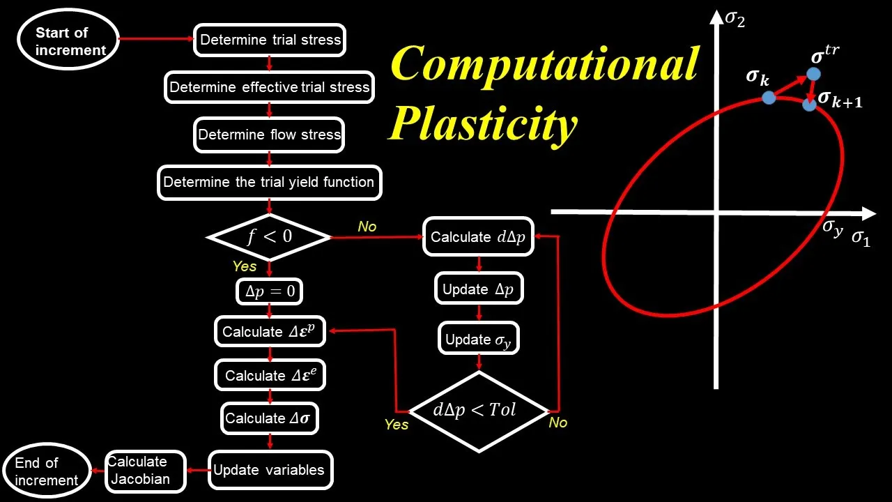
Algorithm

To solve these equations for an increment:

Calculate trial stress or elastic predictor.

Calculate effective trial stress.

Calculate flow stress based on effective plastic strain.

Calculate yield function by effective trial stress and flow stress.

If f is negative, material is elastic and plastic strain is zero. Otherwise, use Newton's iterative method to predict delta p or effective plastic strain increment.

Update variables like stress and effective plastic strain.

Introduction

In this section, the speaker introduces the video and encourages viewers to like, comment, and subscribe to their channel for more videos about mechanics and simulations.

Video Introduction

The speaker welcomes viewers to the video.

The speaker encourages viewers to like or comment on the video.

The speaker asks viewers to subscribe to their channel for more videos about mechanics and simulations.

What is a Simulation?

In this section, the speaker defines what a simulation is and provides examples of how it can be used in various fields.

Definition of Simulation

A simulation is a computer program that models real-world scenarios.

Simulations are used in various fields such as engineering, medicine, and finance.

Simulations can be used to test hypotheses or predict outcomes.

Types of Simulations

In this section, the speaker discusses different types of simulations that exist.

Types of Simulations

Physical simulations model real-world objects or systems.

Mathematical simulations use equations to model systems or phenomena.

Agent-based simulations model individual agents interacting with each other in a system.

Advantages of Simulations

In this section, the speaker explains why simulations are useful tools in various fields.

Advantages of Simulations

Simulations can be used to test hypotheses without risking damage or harm in real life scenarios.

Simulations can save time and money by reducing the need for physical testing or experimentation.

Simulations can provide insights into complex systems that may not be easily observable in real life scenarios.

Disadvantages of Simulations

In this section, the speaker discusses some of the limitations and drawbacks of simulations.

Disadvantages of Simulations

Simulations are only as accurate as the data and assumptions used to create them.

Simulations may not account for all variables or factors that can affect real-world scenarios.

Simulations may be limited by computational power or resources.

Conclusion

In this section, the speaker concludes the video by summarizing key points about simulations.

Summary

A simulation is a computer program that models real-world scenarios.

There are different types of simulations such as physical, mathematical, and agent-based simulations.

Simulations have advantages such as being able to test hypotheses without risking harm or damage in real life scenarios, saving time and money, and providing insights into complex systems.

However, there are also disadvantages such as limitations in accuracy due to data and assumptions used, not accounting for all variables or factors that can affect real-world scenarios, and being limited by computational power or resources.