14 Declarations Feedback

How to Declare Constants and Variables in Programming

Introduction to Data Object Declarations

• The session focuses on declaring constants, variables, structures, and internal tables using various data types.

• Emphasis is placed on SLP rules for naming data objects: names must start with a letter (A-Z), can be up to 30 characters long, and may include alphanumeric characters and underscores.

Creating Constants

• The instructor begins by creating four constants, starting with the maximum integer value. Naming conventions are followed: "constant" is global and prefixed with "GE".

• The minimum integer value is declared similarly; values are assigned after determining the maximum integer from an external source.

• A constant for Pi is created using float type (type F), demonstrating how to specify decimal places.

Defining Variables

• Discussion shifts to defining variables from predefined types visible across all programs. Predefined types can be used for local data types and interface parameters.

• Integer variables are introduced as counters or indexes. Global variable naming convention includes prefixes like "GV" for global variable.

Numeric Types Declaration

• An example of declaring an integer variable with a default value is provided.

• Floating-point numbers are declared next, showcasing how to define them as picked numbers with specified decimal places.

Character Types and Other Data Types

• Character fields that contain alphanumeric characters are defined; single character declarations versus multi-character declarations (up to 255).

• Numeric text fields are discussed as useful in database tables for key values; examples of declaration provided.

Date and Time Fields

• Date fields can be declared in two ways based on required information. The term "datum" is explained as derived from German meaning date.

• Time variables follow similar declaration patterns, reinforcing consistency in naming conventions.

Hexadecimal Types and Strings

• Hexadecimal types interpret individual bytes in memory; their declaration method is outlined.

• Variable-length strings are introduced along with their definitions, emphasizing flexibility in programming.

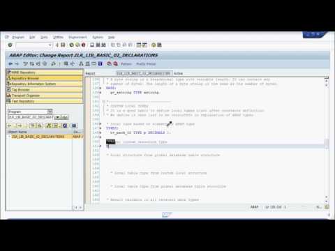
Custom Local Types Definition

• The importance of defining custom local types immediately after constants is highlighted. A new type based on elementary above type is created as an example.

Creating Local Structures and Types in SAP

Understanding Local Custom Structures

• The speaker introduces the concept of local custom structures, explaining that they can hold multiple values within a single variable.

• A local structure is defined with three fields: field one (type C), field two (local type TV), and field three (type ad).

Global Structure Integration

• The speaker discusses declaring a local structure from a global database table structure, using DD 0 to L as an example.

• It is clarified that the TS global structure will contain the structure of the DD 0 to L database table, emphasizing its complexity.

Creating Table Types

• The concept of a local table type is introduced, which functions like a regular database table but exists only in memory during runtime.

• Instructions are provided on how to declare a local table type from a custom local structure.

Utilizing Global Database Tables

• The process for declaring a local table type from global database tables is explained, specifically referencing standard tables like DD 0 to L.

• The importance of using global structures over creating new ones is emphasized for efficiency.

Transitioning to Main Program Logic

• The speaker transitions into discussing main program logic focusing on date and time variables.

• An example is given where current date retrieval and arithmetic operations on dates are demonstrated using specific variable types.

Understanding Data Types and Conversions in Programming

Working with Time Variables

• The speaker explains the use of data types for calculations, specifically focusing on time. They demonstrate how to display time on screen using a variable that holds the value of 90 minutes converted into seconds.

• To calculate 90 minutes in seconds, they multiply by 60, resulting in 5400 seconds. This value is assigned to a variable named GV_time.

• The output is displayed using the GV_time variable formatted as hours, minutes, and seconds.

Displaying Numeric Variables

• The speaker discusses displaying numeric variables rounded appropriately. They perform division (3 divided by 4) to illustrate how different numeric types are represented.

• An integer variable (GV_integer) is created from the result of the division, while a float variable (GV_float) retains its decimal format.

• A picked number with two decimals is also defined and displayed alongside other numeric types.

Structuring Data

• The speaker introduces local structures and demonstrates how to define fields within these structures. They utilize control space for field options.

• Values are assigned to various fields based on their data types: type C for strings, type P for picked numbers (like Pi), and type D for dates.

Outputting Structured Data

• The values from the local structure are outputted on screen using appropriate syntax. Control space assists in ensuring correct field references.

• Syntax checks are performed before executing code to ensure proper formatting and functionality.

Conversion Rules Between Data Types

• The speaker highlights conversion rules between elementary data types, referencing an external link provided in the program outline.

• Various variables are declared to hold results of conversions from one data type to another (e.g., converting a picked number into float).

• Results show successful conversions; however, some limitations arise when representing certain numbers as characters or dates.

This structured overview captures key concepts discussed in the transcript regarding programming with data types, their manipulation, and conversion processes.

Understanding Data Types and Their Positions

The Positioning of Data Types

• Each data type begins at position 40, although the initial characters are not visible. This is crucial for understanding how different types of numbers are represented in programming.

• The concept of "pecked number" is introduced, which relates to how floating-point and integer values are managed in memory.

• When outputting integers on a screen, it’s important to recognize that their representation starts from this specific position, affecting how they are displayed.

• Understanding these positions helps clarify why certain data types behave differently when processed or displayed in programming environments.