Representación de funciones

Understanding Functions: Different Representations

Introduction to Functions

• The course begins with an introduction to functions, focusing on different ways to represent them. An example discussed is the square of a number.

Analytical Expression of Functions

• The analytical expression is described as a formula that represents a function. It relates two sets of real numbers, denoting input (x) and output (y).

• A function is defined as a relationship between two sets, specifically the set of real numbers for both input and output.

Function Representation through Formulas

• The function can be expressed analytically as f(x) = x^2 , indicating that each input value (x) will be squared.

• This representation can also be written as y = x^2 .

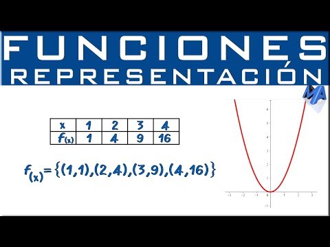
Tabular Representation of Functions

• Another way to represent functions is through tables, where specific values are assigned to x and their corresponding outputs are calculated by squaring those values.

• Commonly used values for x include -3, -2, -1, 0, 1, 2, and 3; however, any real number can be used.

Calculating Outputs from Inputs

• The output values depend on the chosen inputs. For instance, if x = 2 , then f(2) = 2^2 = 4 .

• Continuing this process for other inputs like x = 3 , we find that f(3) = 3^2 = 9 .

Working with Negative Numbers

• When calculating squares for negative numbers such as -2:

• The calculation shows that f(-2) = (-2)^2 = 4 .

• This illustrates how squaring negative numbers results in positive outputs.

Ordered Pairs Representation

• Finally, functions can also be represented using ordered pairs. Each pair consists of an input value and its corresponding output.

Understanding Ordered Pairs and Graphing Functions

Introduction to Ordered Pairs

• The concept of ordered pairs is introduced, emphasizing that the first element (x) is written before the second element (fx). For example, if the first pair corresponds to -2 and 4, it is expressed as (-2, 4).

Characteristics of Ordered Pairs

• It is noted that some values correspond to specific outputs; for instance, at least one input corresponds to 1. The discussion highlights how ordered pairs can continue indefinitely, often ending with ellipses to indicate more pairs exist.

• The importance of maintaining order in these pairs is stressed. An example illustrates that one cannot mix values incorrectly; for instance, pairing 3 with 5 when it should correspond to a different output.

Graphical Representation of Functions

• The graphical method for expressing functions is discussed as one of the most common approaches. A table of values or ordered pairs must be known beforehand.

• A table of values will be created first before plotting on a Cartesian plane. This process involves locating points based on their corresponding x and y coordinates.

Plotting Points on a Graph

• Specific examples are provided for plotting points such as (-2, 4), where -2 represents the x-coordinate and 4 represents the y-coordinate.

• Additional points are plotted sequentially: (-1, 1), (0, 0), (2, 4), and so forth. The speaker notes limitations in displaying all points due to space constraints.

Connecting Points and Function Types

• After plotting points on the graph, they are connected to form a visual representation of the function being analyzed.

• Future videos will focus on different types of functions like linear and quadratic functions. A practice exercise involving writing an analytical function in various forms is also mentioned.

Creating Value Tables

• Viewers are encouraged to create value tables based on given equations like f(x)=2x. They can choose any numbers for x but must multiply them by two for corresponding fx values.

• Examples illustrate how negative inputs yield negative outputs while positive inputs yield positive results. This section emphasizes understanding relationships between variables through graphical representation.