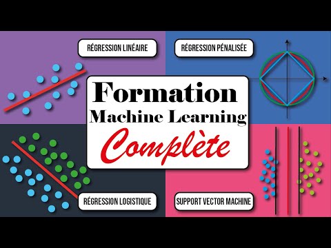
Les modèles que vous devez absolument connaître en Machine Learning

Name: Les modèles que vous devez absolument connaître en Machine Learning
Uploaded: 2023-07-27T08:13:49.000Z
Duration: 4 h 12 min 38 s

Introduction to Linear Algorithms

Overview of the Course

The speaker introduces a new training course focused on linear algorithms, emphasizing their importance in machine learning.

Understanding linear algorithms is crucial for data scientists as they are widely used for regression and classification problems.

The course will cover various topics including linear regression, logistic regression, penalized regressions (L1 and L2), kernel regressions, and support vector machines (SVM).

Course Structure

Each algorithm will have a dedicated video covering theory, implementation from scratch using Python, and usage with Scikit-learn.

A web version of the training is available for free, providing access to all resources used in the course.

Engagement and Support

Community Interaction

Viewers are encouraged to like the video and subscribe to help spread awareness of the training.

The speaker invites comments for questions or feedback during the course, promising to read and respond to them.

Linear Regression Theory

Understanding Linear Regression

The first topic covered is linear regression; it’s defined as a supervised learning algorithm used for predicting continuous variables.

An example given is predicting house prices based on features such as surface area, number of rooms, and year built.

Data Representation

A labeled dataset includes explanatory variables (X), which provide information about the problem being solved.

For simplification in examples, only surface area will be used as an explanatory variable to predict house prices.

Visualizing Relationships

Graphical Representation

The relationship between surface area and price can be visualized with a scatter plot where each point represents a house's attributes.

A trend line can be drawn indicating that price tends to increase with larger surface areas.

Mathematical Model of Linear Regression

Equation Formulation

The mathematical expression for this relationship follows the form y = W_0 + W_1x_1 , resembling affine functions studied previously.

In general cases with multiple explanatory variables, coefficients W_n represent weights applied to each variable in predictions.

This structured approach provides clarity on key concepts discussed throughout the transcript while allowing easy navigation through timestamps linked directly to specific content segments.

Understanding Cost Function and Gradient Descent

Choosing Parameters for the Model

The discussion begins with the challenge of selecting parameters to define a line that helps solve a problem, emphasizing that there are infinite possible parameters leading to numerous lines through two points.

The concept of prediction error is introduced, defined as the distance between the actual price (represented by a blue point) and the estimated price from our model (depicted by a red line).

The goal is to find a line that minimizes this prediction error. Visual representation aids in quantifying errors when only one explanatory variable and few data points are available.

Understanding Cost Function

A cost function estimates the prediction error of the model, calculated as the average distance between predicted values ( haty ) and actual values ( y ).

An example illustrates how to compute average error: if predictions deviate from actual prices, squaring these differences ensures all errors remain positive, preventing cancellation during summation.

Testing Different Models

To refine parameter selection, various models can be tested against their associated errors; choosing the model with minimal error becomes essential.

The mathematical expression for the model is reiterated, fixing W_0 at zero while optimizing W_1 . A cost function graph will illustrate different costs associated with varying W_1 .

Visualizing Cost Function

Starting with W_1 = 0 , initial costs are visualized on a graph. As W_1 increases (e.g., testing values like 0.5 or 1), corresponding costs are recorded.

When W_1 = 1 , it indicates an optimal fit where cost equals zero. Further tests reveal how increasing W_1 affects estimation accuracy.

Challenges in Multi-Dimensional Parameter Space

Exploring multiple parameters simultaneously requires three-dimensional graphs; however, adding more variables complicates visualization beyond three dimensions.

Testing all potential parameter values can be computationally intensive; thus, an analytical approach using gradient descent is proposed.

Introduction to Gradient Descent Algorithm

Gradient descent aims to optimize parameters by iteratively adjusting them based on minimizing cost functions.

The formula for updating parameters involves subtracting a fraction (learning rate between 0 and 1) of the partial derivative of cost concerning each parameter from its current value.

Practical Application of Gradient Descent

Initial random values for parameters lead to iterative updates aimed at minimizing cost over time. This process may seem abstract initially but becomes clearer through practical examples.

Understanding Gradient Descent and Learning Rate in Linear Regression

The Role of Partial Derivatives in Weight Update

To update the weight W1 at time T1 , we need to determine the value of the partial derivative, which represents the slope of the tangent line at that point. A positive slope indicates an increasing function.

The learning rate is a positive number between 0 and 1. Multiplying a positive number (the learning rate) by another positive number results in a smaller adjustment to W1 , leading to a decrease in its value at T1 .

If W1 starts on the opposite side of the slope, it will still move towards minimizing cost. An example shows starting with W1 approx 0 and an associated cost close to 2.3.

Calculating Cost and Adjusting Weights

When applying gradient descent, if the partial derivative is negative (indicating a decreasing tangent), multiplying it by a positive learning rate yields a negative adjustment, effectively increasing W1 .

This new value of W1 at time T1 will be greater than its previous value at time T0. The goal is to repeat this process until convergence towards minimum error.

Convergence Towards Minimum Error

As we approach minimum error, the partial derivative decreases because the slope becomes less steep. Eventually, when reaching uniformity (a flat line), updates cease as derivatives approach zero.

The diminishing size of updates means that as we near our global minimum for cost function J(W), adjustments become increasingly small.

Impact of Learning Rate on Model Convergence

A constant learning rate between 0 and 1 controls weight updates during training. If too large, it may prevent convergence; if too small, convergence can be excessively slow.

It’s preferable to have a smaller learning rate for stable convergence rather than risking divergence with larger rates that could destabilize model training.

Practical Implementation Insights

Understanding theory alone isn't sufficient; practical implementation solidifies comprehension. Upcoming content will focus on coding these concepts from scratch using Python.

Implementing algorithms manually enhances understanding deeply; thus, hands-on coding will commence shortly after importing necessary libraries for matrix operations.

Data Preparation for Linear Regression

Data used for predicting company revenue is accessible via Google Drive links provided in resources. Users can either download or link directly through Google Colab or Jupyter Notebook.

The dataset includes explanatory variables such as city population and ratings affecting revenue predictions. Visualizing these relationships is crucial before proceeding with normalization techniques discussed later.

This structured overview captures key insights from discussions about gradient descent mechanics, weight adjustments based on derivatives, implications of learning rates on model performance, and practical steps toward implementing linear regression algorithms effectively.

Initialization of Linear Regression Class

Class Initialization and Weight Setting

The first function in the class is the initialization function, which requires minimal information, specifically the dimension of the training set to initialize model weights.

A constant random value is assigned to n + 1 parameters, where n represents the number of variables in the training set, ensuring that an intercept is included.

Predict Function Implementation

The next significant function is predict, which calculates the target variable by multiplying explanatory variables with their respective initialized weights.

Initial predictions are checked for correctness; each example should yield a prediction. The use of hstack and a matrix of ones is explained for dimensional consistency during matrix multiplication.

Matrix Operations and Cost Function

Matrix Multiplication Techniques

To perform matrix multiplication correctly, an additional column of ones is added to the training matrix, allowing for efficient computation without altering results mathematically.

The mean squared error (MSE) will be used as a cost function, with both mathematical and vectorized expressions provided to enhance computational efficiency by avoiding loops.

Vectorization Benefits

Vectorized expressions reduce computation time significantly compared to traditional looping methods while maintaining mathematical integrity. This approach allows for faster calculations during model training.

Training Process: Fit Function

Gradient Descent Algorithm

The fit function implements gradient descent to optimize weights based on available data, aiming to minimize the cost function through iterative updates over several iterations defined by a learning rate and iteration limit.

An historical record of costs at each iteration is maintained to visualize performance improvements throughout training sessions. After several iterations, costs should decrease towards zero indicating effective learning from data inputs.

Learning Rate Impact Analysis

Different learning rates (0.1, 0.01, 0.001) are tested; despite slower convergence with lower rates, all models eventually reach similar cost levels demonstrating robustness in learning capabilities across varying rates.

Conclusion on Implementation Practices

Practical Considerations in Machine Learning

While implementing linear regression from scratch serves educational purposes well for understanding fundamentals, it may not match optimizations found in professional libraries like Scikit-learn which offer more efficient implementations suitable for production environments.

Why Normalize Data Before Training?

Importance of Normalization

The video discusses the necessity of normalizing data before training models, explaining that normalization helps address various issues encountered when data is not standardized.

It introduces the use of StandardScaler from Scikit-learn to normalize data effectively, emphasizing its role in preparing datasets for linear regression modeling.

Data Preparation Steps

The presenter outlines steps for importing necessary packages and linking Google Drive to access datasets without needing shortcuts.

A critical risk of training a model on non-normalized data is highlighted: convergence issues can arise, leading to unstable model performance.

Convergence Issues Explained

An example illustrates how error remains constant or even explodes during iterations when using non-normalized data, with cost values reaching extreme levels (10^298).

The increasing error indicates that the scale of variables is too large, causing gradients to diverge significantly and preventing convergence.

Solutions Through Normalization

To mitigate these issues, scaling down variable values (e.g., dividing by 1000) is suggested; this does not alter distributions but improves numerical stability.

After normalization, the model shows improved performance with decreasing costs per iteration, indicating effective learning.

Interpreting Model Coefficients

The importance of understanding coefficients in relation to their respective variables is discussed; without normalization, interpreting these weights becomes challenging due to differing scales.

Normalizing ensures that coefficients can be accurately interpreted since they are now on a comparable scale.

Implementing StandardScaler Correctly

The video demonstrates how to initialize StandardScaler, compute means and standard deviations for normalization, and apply these transformations correctly across datasets.

A common mistake among students—normalizing both training and test sets separately—is addressed. This practice leads to discrepancies in mean and standard deviation between datasets.

Best Practices for Model Training

It’s emphasized that one should only initialize StandardScaler once during training and then apply it consistently across any dataset used later for testing or validation.

Post-normalization results show no further convergence problems during training; errors decrease steadily with each iteration as the model learns effectively.

Normalization of Variables in Linear Regression

Importance of Normalization

The speaker emphasizes that normalizing variables is crucial before training a model, as it ensures that differences between parameters are solely due to interactions with the target variable.

It is highlighted that this principle applies to all linear models discussed throughout the video series.

Transitioning to Model Training

The speaker mentions the transition from implementing linear regression from scratch for educational purposes to using optimized libraries like Scikit-learn for practical applications.

The process begins by importing necessary packages and separating explanatory variables from the target variable, followed by splitting data into training and testing sets.

Model Initialization and Training

Instructions are provided on how to initialize, train, and utilize the linear regression function, which involves storing it in an object called linreg.

To train the model, only explanatory variables and the target variable need to be provided, making it a straightforward process similar to previous implementations.

Performance Evaluation

After training, predictions are made on both training and validation datasets to analyze model performance.

The mean squared error is calculated for both datasets; this step demonstrates how easily one can initialize, train, and use a linear regression algorithm.

Hyperparameters Overview

Discussion on hyperparameters begins with fit_intercept, which determines if there will be an intercept in the model. Default is true unless there's a specific reason not to include it.

The parameter normalize is mentioned but discouraged for use since it's being deprecated in future versions of Scikit-learn.

Additional Hyperparameters

The copy_X parameter allows working on a copy of the dataset rather than modifying it directly; it's recommended to keep this default setting.

The n_jobs parameter controls CPU core allocation during training; setting it to -1 utilizes all available cores for faster processing.

Coefficient Constraints

Lastly, the positive hyperparameter forces all coefficients in the model to be non-negative. It's advised not to use this unless there's a compelling reason as it's rarely applied practically.

Attributes of Linear Regression Model

Key attributes include:

coef_: Accesses different coefficients of your model.

intercept_: Provides access to the intercept value (y-intercept).

Other attributes like rank and singular values are noted but considered less significant.

Understanding Logistic Regression

Overview of Linear and Logistic Regression

The video concludes the discussion on linear regression model training, highlighting the use of functions to retrieve variable counts and names from datasets.

It introduces logistic regression as a new algorithm, contrasting it with linear regression which predicts continuous variables.

The focus shifts to classification problems where logistic regression is used to predict discrete outcomes, such as whether an email will be opened.

Application of Logistic Regression

An example is provided where the goal is to predict email openings based on customer data, using explanatory variables (X) to forecast a binary outcome (Y).

Visualization techniques are discussed for representing customers based on their average basket size and email opening frequency, distinguishing between those likely to open emails (blue points) and those who are not (red points).

Mathematical Foundations

The mathematical expression remains similar to linear regression but aims at classifying observations rather than predicting continuous values.

In logistic regression, predictions yield probabilities between 0 and 1; thus, a sigmoid function is employed to map outputs accordingly.

Cost Function in Logistic Regression

The sigmoid function's graphical representation shows that its output is constrained between 0 and 1. This allows for probability estimations regarding class membership.

The cost function must be minimized differently due to the nature of logistic regression; it becomes non-convex with potential local minima.

Error Classification and Cost Minimization

A new cost function formulation addresses classification errors by ensuring predictions align closely with actual outcomes while minimizing costs associated with incorrect predictions.

When predicting classes, if the prediction matches reality (e.g., Y = 1), the cost is zero; however, discrepancies lead to infinite costs under certain conditions.

Finalizing Cost Function Expression

The final expression for the cost function combines conditions into a single formula that simplifies calculations while maintaining accuracy in error assessment.

This unified approach ensures that when one condition holds true (e.g., Y = 1), irrelevant parts of the equation drop out, streamlining computations for optimization purposes.

By following this structured outline with timestamps linked directly to key insights from the transcript, readers can easily navigate through complex concepts related to logistic regression.

Logistic Regression Implementation in Python

Overview of Logistic Regression

The video discusses the mathematical expression for logistic regression and references a previous video for a detailed demonstration. Viewers are encouraged to watch it if they are interested in mathematics.

The presenter emphasizes that with theoretical knowledge, viewers can implement logistic regression from scratch using Python.

Data Preparation

The dataset used is related to breast cancer, aiming to determine whether a patient has cancer based on provided data. The dataset serves as a test case for function implementation.

Data is separated into explanatory variables (X) and the target variable (y). Standardization of data is performed by subtracting the mean and dividing by the standard deviation.

Class Initialization and Functionality

The initialization function of the logistic regression class requires minimal information, primarily focusing on the dimensions of explanatory variables.

A column of ones is added to the training matrix to facilitate matrix multiplication with weight parameters, ensuring compatibility in dimensions.

Prediction and Cost Function

Predictions generated by the model fall between 0 and 1 due to the use of a sigmoid function, which aligns with expected outcomes.

The cost function implemented is cross-entropy loss. The mathematical expression remains consistent with prior explanations, simplifying coding efforts.

Model Fitting and Training

The fit function incorporates gradient descent algorithms to optimize weights based on available data while minimizing cost functions.

Historical costs during training are tracked; ideally, costs decrease over iterations until reaching a plateau similar to linear regression models.

Learning Rate Impact

Different learning rates (0.1, 0.01, etc.) affect training speed but ultimately lead models toward similar convergence points despite varying initial speeds.

Transitioning to Scikit-Learn

While educational implementations provide foundational understanding, they may not be as optimized as established libraries like Scikit-learn.

Future videos will cover how to train logistic regression models using Scikit-learn while explaining hyperparameters and attributes available for effective model training.

Practical Steps in Scikit-Learn Implementation

Initial steps include importing necessary packages and datasets while separating explanatory variables from target variables for consistency checks before proceeding with normalization.

This structured approach provides clarity on implementing logistic regression from scratch in Python while also preparing viewers for more advanced applications using Scikit-learn.

Training Specialized Models with Logistic Regression

Model Training and Prediction

The fit function is used to train models with the provided data, while the predict function returns the class membership for each observation.

The logistic regression model can also provide probabilities of class membership using the predict_proba function, which shows probabilities for both classes in a classification problem.

Hyperparameters Overview

The hyperparameter penalty is set to 'none' when training a logistic regression model; further discussion on this will occur in future videos.

The dual hyperparameter determines whether to use primal or dual implementation; it’s rarely needed unless specific cases arise.

Stopping Criteria and Default Settings

The tol hyperparameter defines when training should stop based on minimal improvement in cost function; it's advisable to keep it at default unless optimization is critical.

If aiming for quick training, increasing the value of tol may be beneficial, while decreasing it can optimize performance.

Handling Imbalanced Data

The class_weight parameter is crucial for handling imbalanced datasets where one class significantly outnumbers another.

By adjusting costs based on class representation, this parameter ensures that all classes contribute equally to the cost function during training.

Random State and Solver Selection

Setting a fixed random state helps ensure consistent results across different trainings by controlling randomness in model initialization.

It’s recommended to retain the default solver for logistic regression unless specific issues arise that necessitate changes.

Iteration Limits and Multi-class Problems

The max_iter hyperparameter sets iteration limits; if convergence warnings appear, increasing this value may resolve issues.

For multi-class problems, keeping the default setting allows automatic adjustment based on whether the problem is binary or multi-class.

Additional Hyperparameters Insights

Parameters like verbose, which provides additional information during training, are often not particularly useful and can be left at zero.

Using warm start allows leveraging previous training results but should generally remain false unless consecutive trainings are intended.

This structured overview captures key insights from the transcript regarding logistic regression modeling techniques and considerations.

Understanding Hyperparameters and Attributes in Logistic Regression

Key Attributes of the Model

The first attribute, class, returns the training classes but is not particularly useful.

The coef_ attribute provides access to coefficients associated with each training variable, arranged in the same order as the variables.

The intercept_ attribute gives the origin value for your model, while other attributes like n_features_in_ indicate the number of variables used during training.

Introduction to Penalized Regression

Many hyperparameters were not explained because they depend on a penalized version of logistic regression rather than basic logistic regression.

Future discussions will focus on penalized regression, which addresses issues related to linear and logistic models.

Overfitting and Underfitting in Machine Learning

Understanding Overfitting and Underfitting

Overfitting occurs when a model performs well on training data but poorly on test data; underfitting happens when it fails to perform adequately on both datasets.

An example illustrates that using a linear model for non-linear problems leads to high prediction error, indicating underfitting.

Identifying Model Performance

A different model may show zero error on training data but high error on test data, signaling overfitting.

The ideal scenario is low error rates on both training and test datasets, indicating correct training.

Complexity of Models and Regularization Techniques

Model Complexity

Initial models use simple linear regression; complexity increases by adding polynomial terms (e.g., squares of features).

Overly complex models can fit any function perfectly (zero error), leading to overfitting.

Introducing Regularization

To combat overfitting, regularization techniques are introduced into the cost function to minimize both prediction error and parameter values.

Lasso Regression: A Solution for Overfitting

Lasso Regression Overview

Lasso regression incorporates a regularization term that penalizes all parameters equally, aiming for simpler models with fewer parameters.

Tuning Regularization Parameters

The regularization parameter (lambda) controls how much penalty is applied; if too small, it has little effect; if too large, it may hinder reducing prediction errors.

Finding Optimal Lambda Values

Testing various lambda values helps identify the one yielding optimal performance on test datasets.

Understanding Regularization in Linear Models

Introduction to Regularization Techniques

The concept of regularization is introduced as a method to prevent overfitting by adding a penalty term to the cost function of linear models.

Ridge regression, also known as L2 regularization, is highlighted as another approach that adds a squared term of parameters instead of their absolute values.

Differences Between Lasso and Ridge Regression

Lasso regression tends to drive less useful parameters towards zero, effectively selecting variables that impact the model significantly.

In contrast, Ridge regression aims for more uniform parameter values without necessarily eliminating any variables entirely.

Elastic Net: A Combination Approach

The Elastic Net model incorporates both L1 (Lasso) and L2 (Ridge) penalties in its cost function, balancing between variable selection and parameter homogeneity.

It features two regularization terms with respective control parameters; one hyperparameter (alpha or L1 ratio) determines the mix between the two types of regularization.

Practical Implications of Regularization

Setting alpha to 0 results in pure Ridge regression while setting it to 1 leads to pure Lasso regression. An alpha value of 0.5 balances both penalties equally.

The discussion extends beyond linear models, noting that logistic regression can also benefit from similar regularization techniques due to issues like underfitting and overfitting.

Summary of Key Concepts

Lasso regression helps reduce coefficients for less useful variables towards zero, making it suitable when many variables are present but not all are necessary.

Ridge regression focuses on ensuring all relevant variables contribute uniformly to predictions when they are all deemed important.

Elastic Net combines both strategies, allowing for effective variable selection while maintaining balanced contributions from selected predictors.

Conclusion and Next Steps

The speaker encourages viewers to ask questions if anything remains unclear and mentions upcoming content focused on implementing penalized regression models using Python from scratch.

A reminder is given about prior discussions on theoretical aspects before transitioning into practical coding examples for various penalized regressions.

Implementing Penalized Linear Regression from Scratch

Introduction to Penalized Linear Regression

The video begins with an overview of implementing various versions of penalized linear regression using Python, emphasizing the importance of importing necessary packages and data.

A new class function named pennlies is introduced, which includes a hyperparameter for penalty to determine whether to initialize a classic model or one that uses Ridge, Lasso, or Elastic Net.

Hyperparameters in Penalized Models

The discussion highlights two key hyperparameters: lambda, which controls regularization in the cost function, and alpha, which balances L1 and L2 penalties specifically for Elastic Net models.

After initialization, all parameters are accessible. The predict function will multiply the explanatory variable matrix by the weight matrix to estimate the target variable.

Cost Function Calculation

The video explains that there are four different cost functions corresponding to standard linear regression, Ridge regression, Lasso regression, and Elastic Net.

It emphasizes that depending on the penalty hyperparameter value, different cost functions will be implemented mathematically.

Model Training Process

The final function discussed is fit, which trains the model. Changes in cost function derivatives affect gradient descent algorithms used for training.

Each version's associated penalty is initialized accordingly; for example, no penalty for standard linear regression while others use their respective expressions.

Testing and Results Analysis

Testing involves evaluating models without penalties as well as with L1 (Lasso), L2 (Ridge), and Elastic Net penalties. Observations indicate limited impact from L1 due to only two significant variables.

In contrast, L2 shows more substantial parameter reduction effects consistent with expectations since it integrates both penalties effectively.

Conclusion and Recommendations

The presenter notes that while the code serves educational purposes, it is not optimized for production-level machine learning tasks; libraries like Scikit-learn are recommended for practical applications.

A recap of previous implementations of penalized linear regression types (Lasso, Ridge, Elastic Net), stressing understanding algorithm mechanics over optimization.

Practical Implementation Steps

Moving into practical implementation within a notebook environment requires importing multiple packages tailored for each type of regression rather than a single generic package.

Data preparation steps include splitting into training/testing sets followed by normalization before diving into specific algorithm functionalities.

This structured approach provides clarity on implementing penalized linear regression techniques while highlighting essential concepts and methodologies discussed throughout the video.

Hyperparameters and Regularization in Regression Models

Introduction to Hyperparameters

The classical light realization does not involve hyperparameters, while regression models like Lasso require the selection of a coefficient alpha.

For Ridge regression, similar initialization is needed for alpha, but it also requires an L1 ratio that balances the impact of L1 and L2 regularization.

Model Training and Predictions

After initializing models, they are trained using the fit method. Predictions are made on both training and test datasets.

The mean absolute error is calculated for each model's predictions, revealing similar performance across different models.

Impact of Regularization Coefficients

A loop is created to train various models with different regularization values (ranging from 0.1 to 10), observing that higher coefficients lead to more parameters being set to zero.

In Ridge regression, increasing the regularization coefficient results in smaller parameter values; excessively high coefficients can lead to all parameters equaling zero.

Elastic Net Regularization

Elastic Net varies two parameters: correlation coefficient and L1 ratio. An L1 ratio of 0 applies only L2 penalty without setting any parameters to zero.

With an L1 ratio of 1, only the L1 penalty applies, resulting in some parameters being set to zero. A balanced ratio (0.5) allows both penalties to influence parameter values.

Overview of Hyperparameters Across Functions

The discussion transitions into hyperparameter documentation for clarity; redundant hyperparameters across functions will not be elaborated upon.

Key hyperparameters include Alpha (regularization strength), fit_intercept (boolean for intercept inclusion), and normalization recommendations.

Additional Hyperparameter Considerations

Other important hyperparameters include max_iter (maximum iterations during training), tol (stopping criteria based on performance improvement), and warm_start (reusing weights from previous training).

Positive boolean forces coefficients to be non-negative; random_state ensures reproducibility during testing phases.

Emphasis on optimizing alpha as it controls model regularization strength effectively across different regression techniques.

Hyperparameters and Model Training in Machine Learning

Understanding Hyperparameters

The solver hyperparameter allows users to select the optimization algorithm for model parameter tuning. It is recommended to use the default setting, which automatically selects the best solver based on the dataset.

The alpha parameter controls the strength of regularization in models like Elastic Net, while L1_ratio balances the impact of L1 and L2 regularization. Values range from 0 (stronger L2) to 1 (stronger L1).

Key parameters for Elastic Net include alpha, which influences regularization strength, and previously discussed parameters are not revisited.

Transitioning to Classification Models

The upcoming video will focus on training penalized classification models using Scikit-learn, highlighting differences from penalized regression functions.

In Scikit-learn, logistic regression uses a single function for all versions, unlike linear regression where each version has its own function.

Data Preparation and Model Initialization

Initial steps involve importing necessary packages and separating data into training and testing sets before normalization using StandardScaler.

For logistic regression, no penalty is applied by setting penalty='none', differing from previous notation where alpha was used as a regularization coefficient.

Regularization Coefficients Explained

In this implementation, Scikit-learn uses a different notation with C representing the inverse of the regularization coefficient (C = 1/alpha). Adjustments must be made accordingly when setting values.

The default solver may not optimize all versions of penalized logistic regressions; thus, switching to a suitable solver like 'liblinear' is essential for effective model optimization.

Training Models and Addressing Convergence Issues

For Elastic Net logistic regression, both C and L1_ratio need specification. Changing solvers may also be necessary for optimal performance.

During model training with .fit(), convergence issues were noted with Elastic Net due to reaching maximum iterations. Increasing max iterations from 100 to 500 resolved these issues.

Model Validation Techniques

After retraining models successfully without convergence problems, predictions are made using .predict() for class assignments and .predict_proba() for probability assessments.

AUC scores are calculated across models; an AUC score of 0.5 indicates random performance while 1 signifies perfect accuracy. Notably, traditional logistic regression showed no errors on training data—indicative of potential overfitting.

Insights on Regularization Impact

As regularization increases (with smaller weights), it becomes evident that similar functions apply across various logistic regression types; new hyperparameters introduced earlier will be discussed further in subsequent sections.

Understanding Regularization and Non-Linear Problems

Regularization Parameters in Linear Models

The regularization parameter c is crucial for penalizing the cost function effectively, as discussed in the video.

The L1 and L2 penalties are weighted by parameters like L1 Raichu in elastic net models, influencing model performance.

Viewers are encouraged to ask questions if any concepts remain unclear, indicating an interactive approach to learning.

Limitations of Linear Models

All previously discussed models are linear and can only address linear problems; however, most real-world issues are highly non-linear.

Future videos will explore methods to tackle complex non-linear problems using the linear models covered so far.

Introduction to Kernel Trick

The kernel trick allows linear models to solve non-linear problems, a concept that will be elaborated on later in the video series.

An example illustrates how certain distributions cannot be separated linearly, necessitating alternative approaches.

Transforming Non-Linear Problems into Linear Ones

A visual representation shows that even with various lines drawn, separating two different shapes (blue triangles and red squares) remains impossible without additional dimensions.

Introducing a new variable can transform a previously non-linear problem into a linear one by providing a threshold for separation.

Utilizing Landmark Points for Separation

By placing a landmark point within data clusters, it creates an additional variable that helps distinguish between different groups based on proximity.

This new dimension allows for effective separation of data points when visualized in three-dimensional space despite appearing non-linear in two dimensions.

Choosing Appropriate Kernels and Hyperparameters

Various kernels exist for calculating similarity between examples and landmarks; three well-known types include:

Quotient Kernel (RBF): Requires defining hyperparameters and normalizing data before use.

Polynomial Kernel: Involves selecting both degree and constant as hyperparameters.

Sigmoid Kernel: Also requires choosing parameters such as alpha (the slope).

Testing Different Approaches

There is no definitive method or hyperparameter choice upfront; experimentation is key. Testing multiple configurations on your dataset will help identify the best-performing model.

Kernel Trick Implementation in Python

Understanding the Kernel Trick

The video concludes with a summary of the kernel trick, emphasizing its utility in solving nonlinear problems using linear models. Viewers are encouraged to explore additional resources online for further understanding.

Practical Implementation of Kernels

Transitioning from theory to practice, the presenter introduces a hands-on approach by implementing kernels in Python to address previously discussed nonlinear issues.

Data Preparation and Model Training

The session begins with importing necessary packages and creating synthetic data instead of using pre-existing datasets. The goal is to develop a model that predicts y based on x through linear regression.

Acknowledgment that linear models may not be suitable for all problems leads to an attempt at implementing the RBF (Radial Basis Function) kernel for better modeling.

Kernel Function Development

The initialization function for the kernel class is created, focusing on defining Sigma as a hyperparameter. This sets up the groundwork for subsequent transformations.

Two functions are introduced: fit, which retains landmark data for future use, and transform, which applies these landmarks to new datasets.

Data Transformation Process

A new dataset is initialized based on input parameters, iterating over landmarks to apply transformations and create a new dataset (new_data) that incorporates these changes.

Testing confirms that the transformation function works correctly, producing expected results with consistent values across observations.

Evaluating Model Performance

After normalizing data and applying the RBF kernel, a linear regression model is trained on this transformed dataset. Observations indicate improved performance compared to previous attempts.

Visual analysis reveals that the model's predictions are no longer linear, showcasing enhanced capability in handling nonlinear relationships effectively.

Exploring Additional Kernels

Introduction of polynomial kernels highlights how only specific functions need adjustment during implementation while other components remain unchanged.

Following normalization and training with polynomial kernels shows promising results; visualizations confirm effective problem resolution capabilities.

Final Kernel Exploration: Sigmoid Kernel

The sigmoid kernel is tested next; adjustments focus primarily on initialization functions and expression changes within the kernel function itself.

Despite random selection of hyperparameters during testing, successful application demonstrates how sigmoid kernels can also resolve nonlinear issues using linear models effectively.

Conclusion & Next Steps

The video wraps up by hinting at upcoming content focused on utilizing Scikit-learn's built-in functions for training models via kernel tricks efficiently.

An overview of available kernels within Scikit-learn reinforces their practicality in achieving similar outcomes as those implemented manually earlier in the series.

Kernel Functions and Support Vector Machines

Overview of Kernel Functions

The speaker mentions a link to various metrics and kernel descriptions, highlighting that the RBF (Radial Basis Function) is primarily used for calculating the kernel rather than transforming datasets.

It is noted that regardless of the library used, such as Scikit-learn, implementations are cleaner in certain contexts. Ridge regression with integrated kernels is mentioned as an example.

Implementing Kernel Functions

The speaker emphasizes the need to code when using kernel functions for linear regression problems but reassures viewers they will be guided through this process.

A recommendation is made to review previous videos for better understanding before proceeding with coding in the current notebook.

Training Models with Kernels

Random data will be generated instead of importing datasets; a linear model will be trained on this data, which may not perform well due to its non-linear nature.

The first function created will store hyperparameters while the second function will define what’s called a "kernel function," utilizing Scikit-learn's RBF kernel instead of manually implementing it.

Visualizing Results

After generating a 100x100 matrix, new data sets are created and models are trained on them. Visualization shows improved problem-solving capabilities with these new datasets.

The implementation of polynomial kernels demonstrates effective problem resolution similar to previous methods, showcasing flexibility in approach.

Advantages of Using Scikit-learn Kernels

By replacing mathematical expressions with Scikit-learn functions, users can easily switch between different kernels without extensive code changes.

This adaptability allows users to solve problems efficiently by simply modifying parameters within their class definitions without rewriting complex mathematical functions.

Upcoming Content on Support Vector Machines

Viewers are informed about upcoming content focusing on support vector machines (SVM), which is described as sophisticated yet complex.

The speaker plans to simplify SVM concepts while providing necessary theoretical background for both classification and regression tasks. Requests for additional theory videos are welcomed from viewers.

Understanding Support Vector Machines and Generalization

Introduction to Classification and Performance

The video begins with a simple classification example, illustrating how a line can separate two populations (blue squares and orange circles).

Despite achieving 100% performance on the training data, the model may misclassify new data points (black square), indicating poor generalization.

Generalization Issues in Models

The discussion highlights that while logistic regression may face generalization issues, Support Vector Machines (SVM) aim for better generalizability by finding optimal separation.

SVM uses support vectors from observations to create a decision boundary that maximizes the margin between classes.

Concept of Margin in SVM

The distance between the decision boundary and support vectors is termed "margin," which SVM seeks to maximize for improved generalization.

A brief mathematical reminder is provided about vector norms and projections, essential for understanding SVM mechanics.

Mathematical Foundations of SVM

The norm of a vector represents its length; this concept applies across dimensions. Projections are crucial when analyzing relationships between vectors.

In separating classes (e.g., orange circles vs. pink squares), the weight vector W plays a critical role in determining class membership based on projections.

Constraints and Classifications

For correct classifications, projections must meet specific constraints relative to the weight vector's norm. This ensures proper classification of both positive and negative examples.

Observations close to the decision boundary influence margin size; smaller projections lead to smaller margins, affecting model robustness.

Enhancing Model Robustness

Increasing projection sizes can allow for smaller norms of W , thus enhancing classification accuracy without compromising performance.

By adjusting constraints related to W , models can be trained more effectively, ensuring that negative examples fall below -1 while positive ones exceed 1.

Decision Boundary Dynamics

The video discusses how decision boundaries are established using weight vectors while considering new examples' positions relative to these boundaries.

Emphasis is placed on ensuring robust predictions by enforcing stricter margins beyond just being above or below zero for different classes.

This structured overview captures key insights into Support Vector Machines as discussed in the transcript, providing clarity on their functionality and importance in machine learning contexts.

Support Vector Machines: Understanding the Theory and Implementation

Key Concepts in Support Vector Machines

The importance of maintaining a greater distance between positive and negative observations is emphasized, focusing on finding parameters W that satisfy equations for each example.

The target variable y can be either -1 (negative example) or 1 (positive example). Multiplying inequalities by -1 reverses their direction, leading to consistent constraints across both positive and negative cases.

A single equation can represent constraints for both positive and negative examples. The error calculation involves summing the minimum between 0 and the expression derived from these inequalities.

To avoid negative values in cost functions, the inequality is multiplied by -1, allowing for a cost function based on the average maximum between 0 and the previous expression.

The cost function incorporates constraints ensuring that negative examples are less than -1 while positive examples exceed 1. An additional hyperparameter C serves as a regularization term to balance model complexity against error importance.

Mathematical Foundations of SVM

The cost function is structured to enforce maximum margins while calculating errors under specified constraints. This dual focus enhances model performance against outliers.

Regularization plays a crucial role; larger values of C emphasize error minimization, whereas smaller values prioritize keeping parameters small. This concept aligns with logistic regression principles.

Gradient descent will be utilized to optimize parameters. The partial derivative of the cost function is split into two parts based on whether expressions fall below zero or not.

When expressions are above zero, derivatives yield results involving regularization terms divided by sample size, marking an essential step in understanding SVM theory's complexity compared to simpler models like regression.

Practical Implementation Steps

Despite its complexity, SVM aims for high performance through stringent generalization constraints. Understanding foundational theories aids in implementing algorithms from scratch effectively.

Transitioning from theory to practice involves coding an SVM algorithm using Python. Initial steps include importing necessary packages and preparing datasets—specifically using iris data focused on petal and sepal lengths.

Data normalization is critical before applying SVM since it operates as a linear model requiring standardized input features for optimal performance during training phases.

Initialization functions will set up training data parameters alongside regularization coefficients similar to those used in linear regression contexts.

Prediction classes will output binary results (0 or 1), determined by matrix multiplication signs rather than probabilities—a key distinction from other classification methods like logistic regression.

This structured approach provides clarity on both theoretical foundations and practical applications of Support Vector Machines, facilitating deeper understanding and effective implementation strategies.

Support Vector Machines Implementation and Hyperparameters

Implementing the Initial Model

A vector was created using a binary approach where it equals 1 when the expression is positive and 0 otherwise. This allows for a straightforward multiplication with the initial expression, yielding a positive value when greater than zero.

The function was tested successfully, leading to the next step of implementing the fit class to train the model. The target variable is copied and replaced with 0.

A vector of ones is added to the training set, facilitating matrix duplication between W (weights) and X (features). History will store costs at each training iteration.

The partial derivative is implemented similarly to previous functions, creating a binary vector that indicates whether expressions are negative or positive.

The model's performance shows a decrease in cost over time until reaching a global minimum, indicating effective learning.

Visualizing Results

Visualization of the decision boundary reveals it maintains an appropriate distance from both distributions, enhancing generalization on new data.

Transitioning from scratch implementation in Python to utilizing Scikit-learn for SVM models emphasizes efficiency and optimization for production-ready models.

Utilizing Scikit-learn for SVM

Introduction to using Scikit-learn’s SVC (Support Vector Classifier), which addresses classification problems effectively compared to manual implementations.

Explanation of hyperparameters available within Scikit-learn's SVC function will be provided later; initial focus on importing packages and generating visual data separation between classes.

Training the Model

The SVC function initializes without hyperparameters first to understand its basic usage before exploring their significance later on.

Model training follows standard machine learning practices using the fit method. Performance visualization shows correct classifications based on color-coded zones representing different classes.

Understanding Hyperparameters

Despite being linear, SVM can solve non-linear problems due to its kernel trick capabilities; understanding these hyperparameters becomes crucial for effective modeling.

Discussion begins on hyperparameter C, which regulates model complexity: larger values minimize prediction error while smaller values reduce parameter values—critical for optimization decisions.

Importance of understanding kernel parameters highlighted; default RBF kernel enables non-linear problem resolution effectively within Scikit-learn’s framework.

Various kernels available include RBF, polynomial, sigmoid, and linear options; users can customize by passing different kernels as hyperparameters during model setup.

Hyperparameters and Attributes in Support Vector Machines

Understanding Hyperparameters

The hyperparameters integrated into the function include gamma and C0, which are essential for RBF kernels. Previous videos have covered these topics extensively.

The "shrekking" step aims to reduce training time by identifying and removing certain elements to simplify the optimization problem. It's recommended to use default parameters initially.

The SVM by default provides class labels but not membership probabilities; adjusting this hyperparameter is crucial if probability estimates are needed, such as in scoring scenarios.

The tol hyperparameter sets a stopping condition for training when performance does not improve significantly over iterations.

The class_weight parameter adjusts the cost of each example based on class imbalance, ensuring that minority classes have an adequate impact during model training.

Additional Hyperparameters

Adjusting the maximum iterations only becomes necessary if the model fails to converge with default settings.

The decision function shape allows for different strategies (OVR vs OVO); it's advisable to keep default values unless specific needs arise.

Setting a random state ensures reproducibility in experiments involving multiple trainings with varying hyperparameter values, helping distinguish performance differences from randomness.

Key Attributes of SVM Models

Important attributes include class_weight, which indicates weights associated with each class, and coef_, which returns model parameters specifically for linear kernels.

Other attributes like dual_coef_ provide coefficients of support vectors in decision functions, while status_ indicates whether the model has converged successfully or encountered issues.

Attributes such as n_support return counts of support vectors per class; however, some attributes may be less relevant or understood without further context.

Transitioning to Regression with SVM

This section concludes with insights on preparing for regression models using Support Vector Machines (SVM), emphasizing that future discussions will focus on implementing SVR (Support Vector Regressor).

A recap highlights previous content on classification models before transitioning into regression techniques using scikit-learn's SVR functionality.

Preparing Data for SVR

Initial steps involve importing necessary packages, generating data, and visualizing it before normalizing data for effective use within SVR functions.

Unlike classification tasks where SVM is used directly, regression problems utilize SVR; thus understanding its unique set of hyperparameters is essential before proceeding with model training.

Kernel Trick in SVR Models

Understanding the Kernel Trick

The model effectively addresses non-linear problems, despite Support Vector Machines (SVM) being inherently linear. This highlights a significant capability of the SVR model.

The integration of the kernel trick within SVM allows it to handle non-linear issues by default, particularly using the RBF kernel.

Various kernels such as polynomial and sigmoid are available for implementation, enhancing the model's flexibility in addressing different types of data.

Hyperparameters in SVR

Key hyperparameters include C, which regulates error minimization; larger values reduce prediction errors while smaller values minimize parameter values.

The tol hyperparameter sets a stopping condition during training; if performance does not improve beyond this threshold over iterations, training halts.

The shrinking hyperparameter aims to decrease training time by identifying and removing certain elements from optimization problems.

Memory Management and Training Iterations

The cache size parameter determines memory allocation for the kernel; it's advisable to keep default settings unless memory issues arise.

Adjusting max_iter, which defines maximum iterations for model training, should only be done when warnings indicate convergence issues.

Optimizing Hyperparameters

Focus Areas for Optimization

When optimizing parameters, prioritize adjusting C (regularization coefficient) and selecting appropriate kernels based on your specific needs.

Attributes Overview

Attributes like class_ hold limited relevance in regression contexts since there are no classes involved.

Other attributes provide insights into model parameters and support vectors but may not always yield significant information.

Conclusion: Mastery of Linear Models

Learning Outcomes

Throughout this series on linear models within machine learning algorithms, viewers have gained insights into various models including linear regression, penalized models, kernel methods, and support vector machines.