Lecture 24: Phonons

Name: Lecture 24: Phonons
Uploaded: 2020-07-18T11:51:35.000Z
Duration: 1 h 48 min 27 s
Description: Einstein and Debye models

Lecture 24: Introduction to Phonons

Overview of Phonons

The lecture introduces phonons, the fundamental excitations of lattice vibrations in solids, contrasting them with photons discussed in the previous lecture.

The speaker emphasizes that this is not a solid-state physics course and suggests that a full understanding of phonons requires further study in that field.

Key Models and Concepts

The discussion will cover the Einstein model, the Debye model, and dispersion relations related to phonons.

A simplified model is presented where atoms in a solid are connected by springs, leading to various possible vibrations within the system.

Understanding Phonons

Phonons represent quantized vibrations of a crystal lattice; multiple phonons exist due to numerous atomic interactions.

The energy associated with these excitations is given by E = hbar omega, where omega is the angular frequency of vibration.

Normal Modes and Their Importance

Normal modes are independent vibrational patterns derived from diagonalizing a symmetric matrix; they play a crucial role in understanding phononic behavior.

Each normal mode behaves like a simple harmonic oscillator, allowing for calculations involving partition functions without crosstalk between modes.

Dispersion Relations Explained

The relationship between angular frequency (omega) and wave vector (k) is critical; it describes how wave oscillation speed varies with wavelength.

A dispersion relation illustrates how vibrational frequency changes as a function of wavelength, which differs from photon behavior (e.g., omega = ck).

Practical Examples and Visualization

Simple examples will be provided to calculate dispersion relations for phonons, highlighting their dependence on crystal structure.

Understanding Density of States and the Einstein Model

Introduction to Density of States

The wavelength can be considered a label, with the wave vector q being its inverse. This relationship indicates that the number of states is dependent on frequency omega .

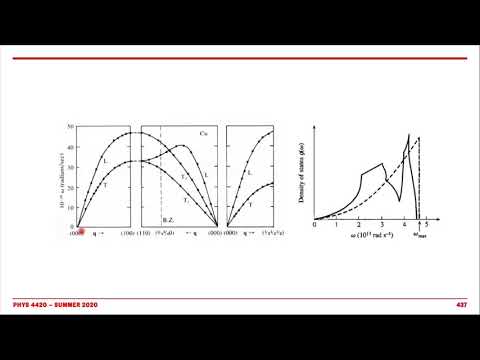
The density of states for materials like copper shows variations with frequency, including increases and dips. A dip occurs in specific frequency ranges, while maxima appear when there are flat bands, indicating many states within a narrow frequency interval.

Key Concepts in Density of States

Understanding the density of states is crucial as it provides priority distribution necessary for calculating the partition function.

Two historical methods will be introduced to model this complex curve related to vibrational states as a function of frequency.

The Einstein Model Explained

The Einstein model simplifies the description of vibrational states by stating that the density of states between frequencies omega and omega + domega can be represented using a Dirac delta function.

This approximation suggests that all modes have the same frequency, termed "Einstein omega," which will be defined further later in the discussion.

Vibrational Modes in Solids

In solids with n atoms, there are typically three vibrational modes per atom due to their connections through springs. However, translation modes reduce this count to 3n - 6 .

While technically correct, for large systems (e.g., one mole), this reduction has negligible impact on calculations since n is extremely large.

Partition Function Calculation

Assuming independent modes allows for straightforward calculation of the partition function as a product across all modes.

The logarithm of this partition function can then be expressed as a sum over individual mode contributions ( z_k ), where each mode behaves like a harmonic oscillator.

Energy Considerations in Oscillators

Each single mode's energy follows quantum mechanics principles; thus, it includes zero-point energy ( n + 1/2 hbaromega ).

Calculating these sums leads to results previously discussed in class regarding thermodynamic properties derived from partition functions.

Understanding the Einstein Model of Solids

Overview of the Einstein Model

The Einstein model assumes that all oscillators in a solid vibrate at a single frequency, which is a rough approximation but simplifies calculations.

Despite its simplicity, this model retains the correct number of modes (3n), leading to results that closely match experimental data.

Density of States and Internal Energy

The density of states plot shows experimental data as a full curve, while the Einstein model approximates it with a single peak.

The internal energy can be derived from the logarithm of the partition function using straightforward calculus techniques.

Transitioning Between Frequency and Temperature

Instead of using angular frequency, it's common to use Einstein temperature (ΘE), linking energy units through Planck's constant and Boltzmann's constant.

This transition involves changing from particle number (n) to molar quantities (R), ensuring equations are applicable per mole.

High Temperature Behavior

At high temperatures, Taylor series expansion allows simplification; when temperature is large, internal energy approaches 3RT, consistent with equipartition theorem results.

This result confirms that including density of states does not alter outcomes significantly at high temperatures due to negligible level spacing effects.

Molar Heat Capacity Calculation

Molar heat capacity is calculated as the derivative of internal energy concerning temperature; for solids, Cp and Cv are similar due to minimal compressibility concerns.

The derivative leads to an equation that remains valid across various temperatures without needing limits for high or low extremes.

Low Temperature Analysis

Understanding Heat Capacity and Models in Statistical Mechanics

Einstein Model Limitations

The heat capacity of a system decreases rapidly, faster than any polynomial growth, leading to discrepancies with experimental data.

At low temperatures, the model struggles to accurately describe low-frequency modes due to its reliance on a single delta peak representation.

In contrast, at high temperatures, the average effects are better captured by the Einstein distribution, yielding a heat capacity of 3R.

Transition to Debye Model

The discussion shifts towards the Debye model, which aims for a more nuanced understanding compared to the Einstein model.

Unlike the Einstein model's delta function approach, the Debye model considers multiple states and their contributions to energy levels.

Phonon Behavior in Debye Model

The Debye model posits that all waves travel at a uniform speed (the speed of sound), simplifying calculations related to phonons.

This assumption leads to a linear dispersion relation where angular frequency is directly proportional to wave vector q.

Density of States Calculation

The density of states can be calculated based on wave vectors; this involves determining volumes within spherical shells in q-space.

The formula for density of states incorporates factors from three possible wave polarizations: one longitudinal and two transverse.

Integration into Partition Function

By equating volume with l^3, we derive an expression for density of states that will be essential for calculating partition functions.

Understanding the Density of States and the Debye Model

The Nature of Density of States

The density of states (DOS) is described as a quadratic term in omega, resembling a parabola. Proper normalization is crucial to ensure that only valid states are represented.

Integration must yield three times the number of particles (3n), which defines the cutoff point known as the Debye frequency.

The Debye Frequency and Its Significance

The red curve represents the Debye model, contrasting with previous models like Einstein's. It provides a better approximation for low-frequency excitations, particularly at low temperatures.

This model allows for straightforward calculations of partition functions, energy, and heat capacity based on the defined density.

Transitioning from Frequency to Temperature

The concept of Debye temperature emerges from converting units related to frequency into temperature terms, indicating maximum phonon frequencies in materials.

Different materials exhibit varying Debye frequencies; stiffer materials like diamond have higher frequencies compared to less stiff ones like neon.

Internal Energy and Heat Capacity Calculations

Internal energy calculations follow similar principles as those used in the Einstein model but utilize a more complex density function derived from earlier discussions.

Heat capacity can be directly measured and calculated using internal energy derivatives. Simplifications lead to an equation that can be analyzed for physical insights.

Analyzing Results from Models

Analysis of Temperature Models

Decay Rates of Temperature Models

The decay rate of the models is discussed, noting that the Einstein model decays too quickly compared to experimental data, while the Dubai model shows a more appropriate behavior.

At low temperatures, the Dubai temperature behaves like a power of T on a logarithmic scale, contrasting with the exponential decay seen in the Einstein model.

High and Low Temperature Behavior

An analytical approach is taken to examine high and low-temperature limits. At high temperatures, beta approaches zero, leading to simplified expressions for heat capacity.

The results from both Einstein and Dubai models yield similar outcomes due to their correct representation of modes in thermal systems.

Low Temperature Calculations

At low temperatures, calculations reveal that heat capacity behaves as 1/x^3 e, aligning closely with experimental expectations and outperforming the Einstein model.

Understanding Dispersion Relations

The discussion shifts towards dispersion relations which describe frequency as a function of wave vector. This relationship is crucial for understanding wave oscillators' behavior based on wavelength.

Newton's Laws and Oscillation Solutions

A single atomic chain model is introduced where displacement from equilibrium positions is analyzed using Newton's second law combined with Hooke's law for springs.

Phonon Dispersion Relation Explained

Deriving the Dispersion Relation

The second derivative respects time, leading to a simplification where the equation involves -omega^2 m multiplied by an exponential term.

The derivation leads to a relationship involving 2 cos(qa), indicating a connection between frequency and wave vector.

This results in a dispersion relation that links frequency (omega) with wavelength (q), crucial for understanding phonons.

Key Parameters in the Model

Constants k, m, and a represent mass, bond strength, and lattice constant respectively, forming the basis of the dispersion relation.

The model indicates that each wave vector corresponds to a specific frequency, essential for phonon behavior analysis.

Visualization of Dispersion Relations

The dispersion relation can be plotted as omega versus q, typically using q for phonons.

A curve representing this relationship is identified as the "first Brillouin zone," although its specifics are not emphasized in this course.

Long Wavelength Limit Analysis

In the long wavelength limit (small q), cos(qa)approx 1 - (qa)^2/2, simplifying calculations significantly.

This approximation leads to a linear relationship between frequency and wave vector at very long wavelengths, indicating low-energy excitations.

Implications of Phonon Models

The linear approximation holds true for low-energy excitations, making it effective for predicting heat capacity at low temperatures.

A visual representation illustrates how longer wavelengths correspond to fewer oscillations; as wavelength decreases, oscillatory behavior increases.

Experimental Data on Phonons

Real-world Applications of Dispersion Relations

Experimental data from materials like copper show complex structures but align well with theoretical predictions near zero energy levels.

Acoustic branches in dispersion relations correlate with sound velocity in materials, highlighting practical applications of these models.

Comparison Between Models

Newton's Second Law and Phonon Modes

Understanding Masses and Spring Systems

Newton's second law is applied to problems involving two types of masses, which can be represented using the same spring system. The analysis mirrors previous discussions on similar systems.

Acoustic vs. Optical Modes

New modes are introduced beyond those previously discussed, including an optical mode that does not approach zero at q = 0 .

Optical modes correspond to oscillations of a dipole moment, which can interact with external electromagnetic fields, allowing for optical excitation.

In contrast, acoustic modes relate to sound propagation in the system and maintain a finite sound velocity even at long wavelengths.

Visualization of Phonon Behavior

An animation from physicsanimation.com illustrates a chain of atoms with different masses, highlighting the behavior of acoustic modes where larger masses move out of phase with smaller ones.

The change in phase between different modes indicates the presence of a dipole moment, reinforcing the concept of optical modes.

Comparison Between Einstein and Debye Models

The Debye model effectively describes low-temperature behavior due to its focus on small frequency excitations associated with acoustic modes.

While the Einstein model may not perform as well overall, it accurately represents sharp peaks corresponding to flat bands in band structure dispersion relations.

Insights into Phonons and Temperature Effects

A phonon is defined as a quantum mechanical excitation related to lattice vibrations; both Einstein and Debye models have been discussed regarding their effectiveness in predicting phononic behavior.

The Einstein model assumes all phonons have identical frequencies but struggles at low temperatures where experimental data shows heat capacity decays as T^3 , unlike predicted exponential decay.

Conclusion on Band Structure Complexity